WIXLIB

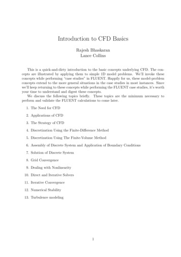
Introduction to CFD BasicsRajesh BhaskaranLance CollinsThis is a quick-and-dirty introduction to the basic concepts underlying CFD. The concepts are illustrated by applying them to simple 1D model problems. We’ll invoke theseconcepts while performing “case studies” in FLUENT. Happily for us, these model-problemconcepts extend to the more general situations in the case studies in most instances. Sincewe’ll keep returning to these concepts while performing the FLUENT case studies, it’s worthyour time to understand and digest these concepts.We discuss the following topics briefly. These topics are the minimum necessary toperform and validate the FLUENT calculations to come later.1. The Need for CFD2. Applications of CFD3. The Strategy of CFD4. Discretization Using the Finite-Difference Method5. Discretization Using The Finite-Volume Method6. Assembly of Discrete System and Application of Boundary Conditions7. Solution of Discrete System8. Grid Convergence9. Dealing with Nonlinearity10. Direct and Iterative Solvers11. Iterative Convergence12. Numerical Stability13. Turbulence modeling1

The Need for CFDApplying the fundamental laws of mechanics to a fluid gives the governing equations for afluid. The conservation of mass equation is ρ · (ρV ) 0 tand the conservation of momentum equation is V ρ ρ(V · )V p ρ g · τij tThese equations along with the conservation of energy equation form a set of coupled, nonlinear partial differential equations. It is not possible to solve these equations analyticallyfor most engineering problems.However, it is possible to obtain approximate computer-based solutions to the governingequations for a variety of engineering problems. This is the subject matter of ComputationalFluid Dynamics (CFD).Applications of CFDCFD is useful in a wide variety of applications and here we note a few to give you an idea ofits use in industry. The simulations shown below have been performed using the FLUENTsoftware.CFD can be used to simulate the flow over a vehicle. For instance, it can be used to studythe interaction of propellers or rotors with the aircraft fuselage The following figure showsthe prediction of the pressure field induced by the interaction of the rotor with a helicopterfuselage in forward flight. Rotors and propellers can be represented with models of varyingcomplexity.The temperature distribution obtained from a CFD analysis of a mixing manifold is shownbelow. This mixing manifold is part of the passenger cabin ventilation system on the Boeing767. The CFD analysis showed the effectiveness of a simpler manifold design without theneed for field testing.2

Bio-medical engineering is a rapidly growing field and uses CFD to study the circulatory andrespiratory systems. The following figure shows pressure contours and a cutaway view thatreveals velocity vectors in a blood pump that assumes the role of heart in open-heart surgery.CFD is attractive to industry since it is more cost-effective than physical testing. However,one must note that complex flow simulations are challenging and error-prone and it takes alot of engineering expertise to obtain validated solutions.The Strategy of CFDBroadly, the strategy of CFD is to replace the continuous problem domain with a discretedomain using a grid. In the continuous domain, each flow variable is defined at every pointin the domain. For instance, the pressure p in the continuous 1D domain shown in the figurebelow would be given asp p(x), 0 x 1In the discrete domain, each flow variable is defined only at the grid points. So, in thediscrete domain shown below, the pressure would be defined only at the N grid points.pi p(xi ), i 1, 2, . . . , NContinuous DomainDiscrete Domain0 x 1x x1, x2, ,xNx 0xx 11xixNGrid pointCoupled algebraic eqs. indiscrete variablesCoupled PDEs boundaryconditions in continuousvariablesIn a CFD solution, one would directly solve for the relevant flow variables only at the gridpoints. The values at other locations are determined by interpolating the values at the gridpoints.The governing partial differential equations and boundary conditions are defined in termsof the continuous variables p, V etc. One can approximate these in the discrete domain interms of the discrete variables pi , V i etc. The discrete system is a large set of coupled,algebraic equations in the discrete variables. Setting up the discrete system and solving it(which is a matrix inversion problem) involves a very large number of repetitive calculations,a task we humans palm over to the digital computer.3

This idea can be extended to any general problem domain. The following figure showsthe grid used for solving the flow over an airfoil. We’ll take a closer look at this airfoil gridsoon while discussing the finite-volume method.Discretization Using the Finite-Difference MethodTo keep the details simple, we will illustrate the fundamental ideas underlying CFD byapplying them to the following simple 1D equation:du um 0; 0 x 1; u(0) 1(1)dxWe’ll first consider the case where m 1 when the equation is linear. We’ll later considerthe m 2 case when the equation is nonlinear.We’ll derive a discrete representation of the above equation with m 1 on the followinggrid: x 1/3x3 2/3x2 1/3x1 0x4 1This grid has four equally-spaced grid points with x being the spacing between successivepoints. Since the governing equation is valid at any grid point, we haveÃdudx! ui 0(2)iwhere the subscript i represents the value at grid point xi . In order to get an expression for(du/dx)i in terms of u at the grid points, we expand ui 1 in a Taylor’s series:Ãui 1Rearranging givesÃdu ui xdxdudx! i! O( x2 )iui ui 1 O( x) x4(3)

The error in (du/dx)i due to the neglected terms in the Taylor’s series is called the truncationerror. Since the truncation error above is O( x), this discrete representation is termed firstorder accurate.Using (3) in (2) and excluding higher-order terms in the Taylor’s series, we get thefollowing discrete equation:ui ui 1 ui 0(4) xNote that we have gone from a differential equation to an algebraic equation!This method of deriving the discrete equation using Taylor’s series expansions is calledthe finite-difference method. However, most commercial CFD codes use the finite-volume orfinite-element methods which are better suited for modeling flow past complex geometries.For example, the FLUENT code uses the finite-volume method whereas ANSYS uses thefinite-element method. We’ll briefly indicate the philosophy of the finite-volume methodnext but will keep using the finite-difference approach to illustrate the underlying conceptswhich are very similar between the different approaches with the finite-difference methodbeing easiest to understand.Discretization Using The Finite-Volume MethodIf you look closely at the airfoil grid shown earlier, you’ll see that it consists of quadrilaterals.In the finite-volume method, such a quadrilateral is commonly referred to as a “cell” and agrid point as a “node”. In 2D, one could also have triangular cells. In 3D, cells are usuallyhexahedrals, tetrahedrals, or prisms. In the finite-volume approach, the integral form of theconservation equations are applied to the control volume defined by a cell to get the discreteequations for the cell. The integral form of the continuity equation for steady, incompressibleflow isZ · n̂ dS 0V(5)SThe integration is over the surface S of the control volume and n̂ is the outward normalat the surface. Physically, this equation means that the net volume flow into the controlvolume is zero.Consider the rectangular cell shown below. x(u4,v4)face 4 yface 1face 3(u1,v1)(u3,v3)face 2y(u2,v2)x5Cell center

The velocity at face i is taken to be V i ui î vi ĵ. Applying the mass conservationequation (5) to the control volume defined by the cell gives u1 y v2 x u3 y v4 x 0This is the discrete form of the continuity equation for the cell. It is equivalent to summingup the net mass flow into the control volume and setting it to zero. So it ensures that thenet mass flow into the cell is zero i.e. that mass is conserved for the cell. Usually, though notalways, the values at the cell centers are solved for directly by inverting the discrete system.The face values u1 , v2 , etc. are obtained by suitably interpolating the cell-center values atadjacent cells.Similarly, one can obtain discrete equations for the conservation of momentum and energyfor the cell. One can readily extend these ideas to any general cell shape in 2D or 3D and anyconservation equation. Take a few minutes to contrast the discretization in the finite-volumeapproach to that in the finite-difference method discussed earlier.Look back at the airfoil grid. When you are using FLUENT, it’s useful to remind yourselfthat the code is finding a solution such that mass, momentum, energy and other relevantquantities are being conserved for each cell. Also, the code directly solves for values ofthe flow variables at the cell centers; values at other locations are obtained by suitableinterpolation.Assembly of Discrete System and Application of Boundary ConditionsRecall that the discrete equation that we obtained using the finite-difference method wasui ui 1 ui 0 xRearranging, we get ui 1 (1 x)ui 0Applying this equation to the 1D grid shown earlier at grid points i 2, 3, 4 gives u1 (1 x) u2 0(i 2)(6) u2 (1 x) u3 0(i 3)(7) u3 (1 x) u4 0(i 4)(8)The discrete equation cannot be applied at the left boundary (i 1) since ui 1 is not definedhere. Instead, we use the boundary condition to getu1 1(9)Equations (6)-(9) form a system of four simultaneous algebraic equations in the fourunknowns u1 , u2 , u3 and u4 . It’s convenient to write this system in matrix form: 1000 1 1 x000 11 x000 11 x6 u1u2u3u4 1000 (10)

In a general situation, one would apply the discrete equations to the grid points (or cellsin the finite-volume method) in the interior of the domain. For grid points (or cells) at ornear the boundary, one would apply a combination of the discrete equations and boundaryconditions. In the end, one would obtain a system of simultaneous algebraic equations withthe number of equations being equal to the number of independent discrete variables. Theprocess is essentially the same as for the model equation above with the details being muchmore complex.FLUENT, like other commercial CFD codes, offers a variety of boundary condition options such as velocity inlet, pressure inlet, pressure outlet, etc. It is very important thatyou specify the proper boundary conditions in order to have a well-defined problem. Also,read through the documentation for a boundary condition option to understand what itdoes before you use it (it might not be doing what you expect). A single wrong boundarycondition can give you a totally wrong result.Solution of Discrete SystemThe discrete system (10) for our own humble 1D example can be easily inverted to obtainthe unknowns at the grid points. Solving for u1 , u2 , u3 and u4 in turn and using x 1/3,we getu1 1 u2 3/4 u3 9/16 u4 27/64The exact solution for the 1D example is easily calculated to beuexact exp( x)The figure below shows the comparison of the discrete solution obtained on the four-pointgrid with the exact solution. The error is largest at the right boundary where it is equal to14.7%.1Numerical solutionExact solution0.90.8u0.70.60.50.400.20.40.60.81xIn a practical CFD application, one would have thousands to millions of unknowns inthe discrete system and if one uses, say, a Gaussian elimination procedure naively to invertthe matrix, you’d graduate before the computer finishes the calculation. So a lot of workgoes into optimizing the matrix inversion in order to minimize the CPU time and memory7