Transcription
ALAQSCFD Comparison of Buoyant andNon-Buoyant Turbulent JetsEEC/SEE/2007/002
ALAQS CFD Comparison of Buoyant and Non-Buoyant Turbulent JetsThis report was prepared for EUROCONTROL Experimental Centre ALAQS by:School of Engineering and Design, Brunel University, UK.Author(s):Syoginus ALOYSIUS, Luiz C. WROBELSchool of Engineering & DesignBrunel UniversityUxbridgeMiddlesexUB8 3PHUKWeb: http://www.brunel.ac.uk/about/acad/sedIan Fuller, EUROCONTROL Experimental CentreReview:ALAQS Peer Review Group.EEC SEE Document Ref.: EEC/SEE/2007/002 European Organisation for the Safety of Air Navigation EUROCONTROL 2007This document is published by EUROCONTROL in the interest of the exchange of information. It may be copied inwhole or in part providing that the copyright notice and disclaimer are included. The information contained in thisdocument may not be modified without prior written permission from EUROCONTROL.EUROCONTROL makes no warranty, either implied or express, for the information contained in this document,neither does it assume any legal liability or responsibility for the accuracy, completeness or usefulness of thisinformation.
ALAQS - CFD Comparison of Buoyant Free andWall Turbulent JetsEXECUTIVE SUMMARYThis report aims to compare the results of CFD simulations of buoyant and non-buoyantturbulent jets, and represents a step towards a better understanding of the source dynamicsbehind airplane jets to provide information for future improvements of existing dispersionmodels. The non-buoyant turbulent jet was first used to validate the CFD code with existingexperimental and analytical results. The same geometry was then analysed with addedbuoyancy to highlight some of the properties that characterise plume rise behind an engine.The method employed to characterise the plume dynamics adopts state-of-the-artComputational Fluid Dynamics (CFD) software packages, which represent the most advancedmathematics that can be applied to the simulation of fluid flow. The Large Eddy Simulation(LES) turbulence model was used to model the smaller eddies present within the grid resolution,and to solve explicitly the large eddies contained outside it.After the successful validation of the non-buoyant jet, the comparison emphasises theimportance of two parameters: the turbulence intensity at the exhaust and the vorticalstructures. They are both interconnected in the definition of the potential core length, which wasfound to be shorter for the buoyant turbulent jet.Three regimes govern the buoyant jet, namely the jet, intermediate and plume regimes. Thenon-buoyant results exhibit only the jet regime.The next step in this research will include ground effects. By progressively reducing thedistance between the jet axis and the ground, important plume dispersion information can becollected which will benefit other dispersion models.
ALAQS CFD Comparison of Buoyant and NonBuoyant Turbulent Jets(This page intentionally blank)ivEEC/SEE/2007/002
ALAQS CFD Comparison of Buoyant and NonBuoyant Turbulent JetsREPORT DOCUMENTATION PAGEReference:Security Classification:SEE Note No. EEC/SEE/2007/002Originator:UnclassifiedOriginator (Corporate Author) Name/Location:School of Engineering and DesignBrunel UniversityUxbridgeUB8 3PHUnited Kingdomhttp://www.brunel.ac.ukEUROCONTROL Experimental CentreCentre de Bois des BordesB.P.1591222 BRETIGNY SUR ORGE CEDEXFranceTelephone: 33 1 69 88 75 00For Society, Environment, EconomyResearch AreaSponsor:Sponsor (Contract Authority) Name/Location:EUROCONTROL EATMEUROCONTROL AgencyRue de la Fusée, 96B –1130 BRUXELLESTelephone: 32 2 729 90 11TITLE:ALAQS CFD Comparison of a Buoyant and Non Buoyant JetAuthors :Syoginus eferences05/0758321828EEC Contact: Ian FullerEATMP TaskProjectTask No. y 2007Distribution Statement:(a) Controlled by:EUROCONTROL Project Manager(b) Special Limitations:None(c) Copy to NTIS:YES / NODescriptors (keywords):ALAQS, CFD, Source Dynamics, Buoyancy Effects, Turbulent Jets, LES, ValidationAbstract:This report aims to compare the results of CFD simulations of buoyant and non-buoyantturbulent jets, and represents a step towards a better understanding of the source dynamicsbehind airplane jets to provide information for future improvements of existing dispersionmodels. The non-buoyant turbulent jet was first used to validate the CFD code with existingexperimental and analytical results. The same geometry was then analysed with addedbuoyancy to highlight some of the properties that characterise plume rise behind an engine.EEC/SEE/2007/002v
ALAQS CFD Comparison of Buoyant and NonBuoyant Turbulent Jets(This page intentionally blank)viEEC/SEE/2007/002
ALAQS CFD Comparison of Buoyant and NonBuoyant Turbulent JetsTABLE OF CONTENTS1INTRODUCTION.12Forthmann Experiment Validation.22.1CFD simulation.22.2Analysis of the Results.52.2.1Axial Velocity Profile for Non-Buoyant Jet.52.2.2Vertical Velocity Profile for Non-Buoyant Jet .82.2.3Theoretical Analysis mien and Goertler theories.10Tollmien solution .10Goertler solution .12Some comments on the theoretical approaches.13Comparison of theoretical and CFD results .14Some Problems with Forthmann’s Experiment .17Buoyant Jets .182.3.1Axial Velocity Profile for Buoyant Jet.182.3.2Vertical Velocity Profile for Buoyant Jet .20Three-dimensional study of free turbulent jet .223.1Geometry and Boundary Conditions.233.2Mean Velocity Profile Comparison.233.3Vorticity Profile 2007/002vii
ALAQS CFD Comparison of Buoyant and NonBuoyant Turbulent JetsLIST OF FIGURESFIGURE 1 - GENERAL DESCRIPTION OF PLANE JET . 3FIGURE 2 - MESH SENSITIVITY RESULTS . 4FIGURE 3 - TWO-DIMENSIONAL JET VELOCITY CONTOURS . 5FIGURE 4 - VELOCITY PROFILE ALONG THE AXIS OF THE JET. 6FIGURE 5 - TURBULENCE KINETIC ENERGY PROFILE ALONG THE JET AXIS . 6FIGURE 6 - VELOCITY PROFILE COMPARISON ALONG THE CENTRE OF THE JET. 7FIGURE 7 - POTENTIAL CORE DESCRIPTION. 8FIGURE 8 - CFD VERTICAL VELOCITY PROFILE COMPARISON AT DIFFERENT DISTANCES BEHINDTHE JET . 9FIGURE 9 - TOLLMIEN VERTICAL VELOCITY PROFILE . 12FIGURE 10 - GOERTLER VERTICAL VELOCITY PROFILE . 13FIGURE 11 - VERTICAL VELOCITY COMPARISON BETWEEN CFD AND THEORETICAL METHODS. 14FIGURE 12 - ANGLE OF SPREAD COMPARISON ABOVE THE CENTRELINE . 15FIGURE 13 - TURBULENCE KINETIC ENERGY COMPARISON AT DIFFERENT DISTANCES BEHINDTHE JET . 16FIGURE 14 - VORTICITY CONTOUR AROUND Z-AXIS WITH ISOLINES (1/S) . 16FIGURE 15 - VORTICITY PROFILE COMPARISON AT DIFFERENT DISTANCES BEHIND JET . 17FIGURE 16 - HORIZONTAL VELOCITY PROFILES WITH AND WITHOUT BUOYANCY . 18FIGURE 17 - VELOCITY PROFILE AT DIFFERENT DISTANCES ABOVE AND BELOW THE JET AXIS. 19FIGURE 18 - VELOCITY CONTOURS FOR BUOYANT JET . 19FIGURE 19 - VELOCITY PROFILE COMPARISON WITH BUOYANCY AT DIFFERENT DISTANCESBEHIND THE JET . 20FIGURE 20 - ANGLE OF SPREAD COMPARISON WITH BUOYANCY JET ABOVE THE CENTRELINE . 21FIGURE 21 - ANGLE OF SPREAD TREND LINE WITH ADDITION OF BUOYANCY. 21FIGURE 22 - VORTICITY PROFILE COMPARISON AT DIFFERENT DISTANCES BEHIND BUOYANT JET. 22FIGURE 23 - GEOMETRY AND MESH DISTRIBUTION OF THE CONTROL VOLUME. 23FIGURE 24 - CENTRELINE AXIAL VELOCITY COMPARISON BETWEEN BUOYANT AND NONBUOYANT JET AT DIFFERENT TIME STEPS. 24FIGURE 25 - MEAN VELOCITY PROFILE EVOLUTION FOR NON-BUOYANT AND BUOYANT JETS. 25FIGURE 26 - ANGLE OF SPREAD COMPARISON AFTER 1S ABOVE THE CENTRE OF THE JET AXIS . 26FIGURE 27 - ANGLE OF SPREAD COMPARISON AFTER 5S ABOVE THE CENTRE OF THE JET AXIS . 27FIGURE 28 - ANGLE OF SPREAD COMPARISON AFTER 10S ABOVE THE CENTRE OF THE JET AXIS . 28FIGURE 29 EVOLUTION OF THE MAXIMUM HEIGHT OF THE PLUME CENTRELINE . 28FIGURE 30 - INSTANTANEOUS VELOCITY PROFILE AFTER 5S FOR THE BUOYANT JET. 29FIGURE 31 - VORTICITY MAGNITUDE AT 5S FOR THE BUOYANT JET. 29FIGURE 32 - Z-VORTICITY COMPARISON AFTER 5S. 308EEC/SEE/2007/002
ALAQS CFD Comparison of Buoyant and NonBuoyant Turbulent JetsABBREVIATIONSCFDComputational Fluid DynamicsBSBell ShapeSRSuccessive RatioRMSRoot Mean SquareTITurbulence IntensityLSLength ScaleALAQSAirport Local Air Quality StudiesNOxNitrogen OxidesLESLarge Eddy SimulationPIVParticle Image VelocimetryEEC/SEE/2007/002ix
ALAQS CFD Comparison of Buoyant and NonBuoyant Turbulent Jets1 INTRODUCTIONThe study of horizontal turbulent jets has been an important and interesting topic for manyyears. An early experimental investigation was conducted by Forthmann (1934) on a planeturbulent jet [Ref 1.]. Since then, progress has been very slow and it is only in the last decadethat extensive research has been conducted on the flow structure of turbulent jets [Ref 2.]. Thissudden interest in the field is due to its wide application in science and engineering. Forinstance, an airplane jet engine emits different types of pollutants. The study of their dispersionwill help dispersion modellers to produce more accurate simulations and predictions to regulateairport traffic.Experimental studies on turbulent flows have increased in accuracy from simple pitot tubemeasurements to complex Particle Image Velocimetry (PIV) photos, but this can be veryexpensive and time consuming for such complex problems. Computational Fluid Dynamics(CFD) has become an alternative to those complicated and laborious works, especially with theincrease in computer technology. Processor speeds have increased at an unprecedented rateand models such as Large Eddy Simulation (LES) can play a major role in understanding theflow behaviour.The basic concept of the LES model is to explicitly solve the larger eddies of the control volume,whereas the smaller eddies are modelled through spatial filtering. Although this model is notsuited for a complete airport simulation at present due to extensive requirements of computerspeed and memory, it can be used efficiently in local studies related to source dynamics andengine plume/wing tip vortex interactions.A LES model was used in this report to investigate the differences between turbulent buoyantand non-buoyant jets in a free atmosphere condition, highlighting the dispersion mechanismbehind the exhaust. The first part of the report aims at validating the CFD simulation withexperimental work in a non-buoyant condition. Analytical results are also derived and comparedto the simulation. Buoyancy effects were then included in the form of a passive species atdifferent density and temperature from the ambient air.EEC/SEE/2007/0021
ALAQS CFD Comparison of Buoyant and NonBuoyant Turbulent Jets2 FORTHMANN EXPERIMENT VALIDATIONThis experiment, conducted in 1934, is the earliest on plane turbulent jets recalled through theliterature [Ref 1.]. The simplicity of its results and the comparison with different analyticalmodels makes it an ideal choice to validate CFD models.Forthmann used a rectangular jet nozzle 0.03m high and 0.65m wide, i.e. with an aspect ratio of21.7, to investigate the free jet expansion. The jet releases an air stream at a velocity of 35m/sinto an unbounded ambient still air. The measurements were taken by a pitot tube whichrecords static pressure of the flow, and the final velocity was computed by using an equation forthe dynamic pressure [Ref 3.].2.1CFD simulationAn extensive research has been undertaken to find the best way to represent the overallgeometry of Forthmann’s experiment, and to conduct the CFD calculations more efficiently. Inhis paper, Forthmann suggested his free jet experiment could be reduced to a two-dimensionalproblem, and compared his results with analytical ones based on the two-dimensionalityapproach of the problem. This approach will be discussed in more detail later in the report.While reducing the geometry to two dimensions, it is important to find out the best controlvolume domain to enclose the flow. This characterisation is closely linked with the boundaryconditions to be assigned on each wall.The boundary conditions were setup as follows: The inlet jet has a velocity of 35m/s. The inlet condition is assigned right at the beginningof the control volume in accordance with the findings of Klein et al. [Ref 4.] and Stanleyet al. [Ref 5.], also reported by Celik et al. [Ref 6.]. The air coming out of the jet isisothermal with the ambient air of the control volume, so that no buoyancy is present inthe simulation. The boundaries just next to the jet were set as walls. The top and bottom boundaries were also assigned as walls. The classical outflow boundary condition is assigned at the outlet.A simple preliminary study confirmed that a control volume of dimensions 4.4m by 3.2m issufficiently large to avoid influences from the artificial boundaries. A proper meshing can now beapplied to the domain, which is mostly refined near the jet exhaust up to a distance of 1mbehind the jet. A mesh sensitivity analysis was then conducted, comprising of three tests withdifferent mesh density by varying the number of grid points and the grid spacing near the jet.The figure and table below show the mesh distribution for each test.It is known from Forthmann’s results that the core of the jet geometry has a bell shape (B.S.)distribution profile. The other edges have a simple successive ratio (S.R.) grading, where thelength of the following edge is multiplied by a constant ratio.2EEC/SEE/2007/002
ALAQS CFD Comparison of Buoyant and NonBuoyant Turbulent Jets21Test123MeshDensity#1155012514,375cellsB.S. 0.45 S.R. 1.04 S.R. 1.0234.4m0.03m#22575200B.S. 0.45 S.R. 1.04 S.R. 1.02#330100250B.S. 0.45 S.R. 1.04 S.R. 1.0235,000cells57,500cellsTable 1 - Mesh Distribution3.2mPotential coreyum2zbxum2b0Flow developmentregionFully developed flowFigure 1 - General description of plane jetThe results presented in Figure 2 are for the velocity profile at a location 0.2m behind the jet fordifferent tests. The graph is non-dimensionalised as follows: The non-dimensional coordinate ( y / b) represents the ratio between vertical position anddistance from the axis to the point at which the velocity is equal to 1um .2The non-dimensional velocity (u / u m ) represents the ratio between local velocity and jetaxis velocity.EEC/SEE/2007/0023
ALAQS CFD Comparison of Buoyant and NonBuoyant Turbulent JetsFigure 2 - Mesh sensitivity resultsThe influence of mesh density on the results can be better seen near the centre of the jet andon the sides of the curve where Test 1 is slightly more pronounced than Test 2, which showsalso some deviation from Test 3 which has a higher mesh density. Thus, the results for Test 3were taken for comparison with Forthmann’s experimental work.Because of the lack of experimental information, the CFD simulation was run long enough toreach a steady state. Another important parameter not mentioned in Forthmann’s paper is thelevel of turbulence coming out of the jet exhaust. The setting of the turbulence parametersincludes the turbulence intensity and its length scale. Wygnanski and Fiedler [Ref 7.] reported intheir study of self-preserving jets a turbulence intensity value of 1%, whereas Deo et al. [Ref 8.]obtained a value of 0.5%. Reviewing some of the experimental work on jets, Rodi [Ref 9.] alsofound a variety of turbulence intensities up to 1%, although some refer to other types of jets.A study was then conducted to observe the data sensitivity when the turbulence intensity andlength scale parameters are modified.1. Turbulence intensityTurbulence intensity is obtained by dividing the RMS value of the velocity component by itsmean value [Ref 10.]. Normally, wind tunnel experiments have very low turbulence intensity butin real conditions such as atmospherical studies this value can reach up to 40% in a suburbanarea near the ground [Ref 11.].Appendix A shows that, even though the differences are very low, the higher the turbulenceintensity the more symmetrical is the predicted behaviour of the jet profile. Moreover, in the nearfield very close to the jet, Forthmann’s experiment suggests a bell shape for the velocity profilein the fully developed region. It can be seen that this shape is very well reproduced with aturbulence intensity of 5%, whereas the other two results show a portion of the potential corewhich still appear to b
Computational Fluid Dynamics (CFD) software packages, which represent the most advanced mathematics that can be applied to the simulation of fluid flow. The Large Eddy Simulation (LES) turbulence model was used to model the smaller eddies present within the grid resolution, and t