Transcription
Comparison of CFD Methods to Wind-tunnel Data for aClass 43 High Speed TrainJustin Morden, Hassan Hemida, Chris BakerSchool of Civil Engineering, University of Birmingham, UK., B15 2TTjam239@bham.ac.ukAbstractThis paper focuses on the application of computational fluid dynamics (CFD) to external aerodynamicflow around a 1/25th scale class 43 HST model. The CAD model of the train featured a high level ofgeometric detail within the under-carriage region to improve the accuracy of the simulation and toprovide a more accurate simulation of under-body and wake flow structures. Two different CFDmethods were used to study the flow around the HST. The obtained surface pressures are compared towind tunnel data previously collected in order to determine the best practice when simulating externalflows.
1IntroductionValidation of the CFD approach is a critical stage prior to any investigation due to the sensitivity ofthe setup to a number of factors. With the power of computers following Moore’s law the optimumsetup used is constantly evolving. With current computational power high detail RANS (Reynoldsaveraged Navier-Stokes) based simulations are becoming the normal, therefore a new more accurateapproach needs to be investigated to continue pushing research forward. Research published for theLES (Large Eddy Simulation) approach has relied upon the use of highly simplified trains that omitunder body detail and even the inter-carriage gap in some circumstances. This research approachprovides a high level of insight into the fundamental flow regimes that occur around the body of atrain at different yaw angles but fail to accurately study the effect of under body details. This paperlooks at the application of a DDES (Delayed Detached Eddy Simulation) approach to a 1/25 scaleclass 43 HST train with a high level of geometric detail around the under-body. The surface pressurecoefficients results of the two CFD approaches will be compared to data collected from a comparablewind-tunnel test to assess their accuracy and allow for a conclusion to be made.2Wind-tunnel experimentWind tunnel tests were conducted by RWDI on behalf of the research project, The tests wereconducted on a 1/25th scale two car model of a class 43 train (Figure 1) on a scale ballast shoulderwith rails (Figure 2) The power car, passenger carriage, inter-carriage gap and bogies were allincluded in the model. The train and ballast shoulder were mounted upon a raised platform 20cmabove ground level to remove any effects created by the boundary layer on the wind tunnel floor. Thepower car was fitted with 313 pressure taps over its surface that were sampled for a time of 120seconds for each run to provide time average results. The power car mount was fitted with a load cellto enable the measurement of lift and drag forces and the overturning moment. A total of 11 runs wereconducted where the trains yaw angle was varied from 00 to 450 in 5 degree increments at a constantflow velocity of 13.2m/s, the Reynolds number for these simulations was to 1.0x10⁵ which is belowthe recommendations made in British Standards (2009) for the conducting of wind tunnel tests.Figure 1: full scale HST.Figure 2: 1/25th scale HST windtunnel model.
3CFDThe initial step in conducting the CFD simulations was the simplification of the CAD geometry; thisinvolved the removal of the windscreen and roof slats due to their minimal importance andcomplexities during the meshing process. The sensor umbilical cord was also excluded from the CADgeometry due to its exact dimensions being unknown.Figure 3: Computational domain sizes (H is height of train)Figure 3 shows the overall domain size. The blockage ratio calculates to be 6% including the raisedplatform, this is below the recommendations in section 5.3.4 of the BS EH 14067-4:2005 A1:2009guidelines which recommends 10%. The blockage ratio of 6% is also lower than the blockage ratiosused in Ekeroth (2009) and Hemida (2009).3.1CFD setupBoth the RANS and DDES setups were initially run using first order upwind schemes before beingswitched to 2nd order central differencing schemes, this approach was chosen to improve the initialstability of the simulation and to reduce the time required to achieve convergence. The DDESsimulation used a Crank-Nicholson 2nd order scheme for the time integration.Convergence for the simulation was determined by monitoring the drag and lift forces of the leadingcarriage until there was no more change against time when plotted using line of best fit using apolynomial of two.For the RANS simulations the SIMPLE algorithm proposed in Szablewski (1973) was used for thepressure-velocity coupling. The DDES experiments used the PISO algorithm proposed in Issa (1986)for pressure-velocity coupling.
3.2Computational MeshMultiple meshes were produced using the Ansys Tgrid software to conduct a mesh sensitivity study(Figure 4), results of the study showed that a fine mesh of 34 million cells (Figure 5) would providethe highest accuracy whilst still ensuring suitable hardware requirements.Figure 4: Mesh sensitivity studyFigure 5: Close up of Fine mesh, showing engine and first bogie (red) and a central slice through the mesh (black)Figure 5 shows a close up of the fine mesh, along the central slice it can be seen how the mesh densityis varied depending upon its location, the mesh near the train is reduced in size in comparison to thelarger cells that can be seen on the left side. Due to the importance of underbody detail on the flowfield around a train as described in Baker (2010) and Jönsson (2010) the mesh is further refinedbetween to ballast shoulder top and the mid axel height.
4ResultsPressure taps fitted to the wind tunnel model are grouped in lines (clips) around the train on all threeaxis, The location of the chossen clip lines for study can be seen in Error! Reference source notfound.6.Figure 6: Clip locations on trainFigure 7: Cp at clip location 1Error! Reference source not found.7 shows surface pressure coefficient around clip location 1, itcan be seen that both the RANS and the DDES approach have similar profiles with the DDES resultspredicting lower pressure coefficients at all locations. Around the train sides and the undercarriage thetwo approaches are within or close to the margin of error for the wind tunnel results. Over the roof theRANS method significantly under predicts the pressure coefficient in comparison to the wind tunnelmeasurements. The DDES method better predicts this, though the calculated value is still below themeasured value and its margin of error. It is worth noting that neither the RANS nor DDES approachpredicted the pressure drops recorded near the lower sides to the train.
Figure 8: Cp at clip location 2Error! Reference source not found.8 shows the surface pressure coefficients at clip location 2, atthis location both CFD methods predicted similar pressure coefficients to each other over the trainsside and roof but differ slightly within the under-body region. Both approaches predict higher pressurecoefficients than recorded however both are nearly entirely within the margin of error for the windtunnel data. Around the lower right side and under carriage the DDES approach proves to be moreaccurate by correctly predicting the drop in pressure whereas the RANS approach predicted a rise inthe surface pressure coefficient.Figure 9: Cp along train centre lineFigure 11 shows a clip along the trains centre line, at this locations the surface pressure coefficientsover the trains roof were calculated as an average of pressure taps that are located in close proxiemtyeach side of the centre line. Along the centre line of the train both approaches predict the surfacepressure coefficients generaly stay within the margin of error for the wind tunnel results. The RANSand DDES results also predict simular surface pressure variations within the under-body region,however a lack of pressure tap points within this location in comparison to the geometric complexityadds uncertainty to any conclusions that could be made.
Figure 10: Cp at clip location 4Figure 11: Cp at clip location 5Error! Reference source not found.10 and 11 shows surface pressure coefficients around the leftside of the train starting at the front centre. Both CFD methods show good correlation with resultsobtained from the wind tunnel tests by remaining within the margins of error for a large majority ofthe results. In Error! Reference source not found.10 it can be seen that the DDES results overpredict the head peak pressure coefficient, the difference between the DDES and RANS results at thispoint are due to differences in predictions of seperation over the ballast shoulders step. In Figure 11both approaches under predict the head peak pressure and the surface presures around the corners ofthe train, this is caused by the removal of the windscreen detail which is normaly recessed causingdisturbance to the flow around its edges.
5ConclusionBoth methods accurately replicated the surface pressure coefficients over the train, generally theDDES approach better predicted peak pressures in comparison to the RANS results. The simularity ofresults was to be expected due to the relative simplicity of calculating surface pressures and due toboth approaches relying upon a RANS approach in the near wall regions. A larger difference in theapproaches could be seen when the drag coefficients were compared to the wind tunnel data, the windtunnel model had a drag coefficient of 0.12 whilst the DDES results calculate the drag coefficient tobe 0.095, This was considerably more accurate than the RANS results that calculate the dragcoefficient to be 0.074. The large difference between the two approaches was due to the difference inwake predictions and the underpredictions of the train head pressure by the RANS approach. Theresults showed that the overall increase in accuracy and flow information obtainable from the DDESsimulation out weighed its increased computational expense when compared to the RANS approach.6BibliographyBaker, C. 2010. The flow around high speed trains. Journal of Wind Engineering and Industrial Aerodynamics,98, 277-298.British Standards. 2009. BS EN 14067-4:2005 A1:2009.Ekeroth, F., Kalmteg, N., Pilqvist, J. & Runsten, J. 2009. Crosswind flow around a high-speed train onembankment.Hemida, H. & Krajnovic, S. 2009. Exploring flow structures around a simplified ICE2 train subjected to a 30degree side wind using LES. Journal of Engineering Applications of Computational Fluid Dynamics.Issa, R. I. 1986. Solution of the implicitly discretised fluid flow equations by operator-splitting. J.Comput. Phys., 62, 40-65.Jönsson, M. 2010. Numerical investigation of the flow underneath a train and the effect of design changes.Menter, F. R. 1994. Two-equation eddy-viscosity turbulence models for engineering applications. AIAA journal,32, 1598-1605.Spalart, P. R. 2009. Detached-eddy simulation. Annual Review of Fluid Mechanics, 41, 181-202.Szablewski, W. 1973. B. E. Launder and D. B. Spalding, Mathematical Models of Turbulence. 169 S. m. Abb.London/New York 1972. Academic Press. Preis geb. 7.50. ZAMM - Journal of Applied Mathematicsand Mechanics / Zeitschrift für Angewandte Mathematik und Mechanik, 53, 424-424.
Comparison of CFD Methods to Wind-tunnel Data for a Class 43 High Speed Train Justin Morden, Hassan Hemida, Chris Baker School of Civil Engineering, University of Birmingham, UK., B15 2TT jam239@bham.ac.uk Abstract This paper focuses on the application of computational fluid dynamic