Transcription
Research articleGeosci. Commun., 1, 25–34, 2018https://doi.org/10.5194/gc-1-25-2018 Author(s) 2018. This work is distributed underthe Creative Commons Attribution 4.0 License.Building a Raspberry Pi school magnetometer network in the UKCiarán D. Beggan1 and Steve R. Marple21 BritishGeological Survey, Research Ave South, Riccarton, Edinburgh, UKDepartment, Lancaster University, Lancaster, UK2 PhysicsCorrespondence: Ciarán Beggan (ciar@bgs.ac.uk)Received: 22 June 2018 – Discussion started: 9 July 2018Revised: 8 September 2018 – Accepted: 24 September 2018 – Published: 10 October 2018Abstract. As computing and geophysical sensor components have become increasingly affordable over the pastdecade, it is now possible to design and build a cost-effectivesystem for monitoring the Earth’s natural magnetic field variations, in particular for space weather events. Modern fluxgate magnetometers are sensitive down to the sub-nanotesla(nT) level, which far exceeds the level of accuracy requiredto detect very small variations of the external magnetic field.When the popular Raspberry Pi single-board computer iscombined with a suitable digitiser it can be used as a low-costdata logger. We adapted off-the-shelf components to designa magnetometer system for schools and developed bespokePython software to build a network of low-cost magnetometers across the UK. We describe the system and software andhow it was deployed to schools around the UK. In addition,we show the results recorded by the system from one of thelargest geomagnetic storms of the current solar cycle.1IntroductionOver the past decade, the introduction of cheap reliable computing hardware and sensors, along with the ubiquity ofhigh-speed Internet connections, mean that it is now possible create low-cost open-science networks of geophysical sensors. This has encouraged the development of dataintensive networks, for example in climate studies (WeatherObservation Website: https://www.metoffice.gov.uk/, last access: 8 October 2018), seismology (BGS School Seismology Project: http://www.bgs.ac.uk/schoolseismology/, lastaccess: 8 October 2018) or cosmic ray research (theTimPix Project: http://www.researchinschools.org/TIMPIX/home.html, last access: 8 October 2018), where spatial andtemporal gaps in the professional scientific networks maybe filled or augmented. Some networks employ existingplatforms such as mobile phones using in-built sensors torecord data (e.g. CrowdMag, see https://www.ngdc.noaa.gov/geomag/crowdmag.shtml, last access: 8 October 2018)while others create bespoke hardware with higher accuracy than general-purpose systems. In geomagnetism, highquality low-cost fluxgate sensors have become widely available, allowing accurate monitoring of the variation of theEarth’s magnetic field over time ranges of several minutesto hours. This prompted us to investigate the various types ofcommercial sensors and their ability to monitor the externalmagnetic field, and in particular their ability to record largegeomagnetic storms.The Raspberry Pi is a small single-board computer thattypically runs the Linux operating system. Peripherals suchas sensors may be directly connected to its general purposeinput–output (GPIO) pins. Relatively cheap fluxgate magnetometer sensors are now available from a number of suppliers and analog-to-digital converters are also commonplace inthe Raspberry Pi ecosystem. For around 1/100 of the price ofa conventional scientific-standard fluxgate magnetometer instrument we found that we could build a system with approximately 1/100 the accuracy and resolution. (At 2018 prices,the Raspberry Pi magnetometer costs around GPB 150.) Despite the lower accuracy, this is still easily sufficient to recordthe daily variation of the Earth’s ionosphere and magnetosphere, in order to detect the rapid changes in the magneticfield during geomagnetic storms. As a combination of a citizen science experiment and an outreach and education programme in geophysics, we applied to the UK Science Technology and Facilities Council (STFC) in 2015 for a SmallPublic Engagement grant and were successful. In the application we bid for funding to build and deploy 10 systems toschools across the United Kingdom.Published by Copernicus Publications on behalf of the European Geosciences Union.
26C. Beggan and S. R. Marple: Raspberry Pi magnetometer networkIn Sect. 2 of this paper we briefly describe the scienceof the magnetic field and what a sensor measurement consists of. In Sects. 3 and 4 we outline how our system worksand was deployed to create a school network. As an example of its utility for science, in Sect. 5 we show the resultsof combining the Raspberry Pi magnetometer network withmeasurements from the permanent magnetic observatory network in the UK to enhance our understanding of the spatialand temporal dynamics of a large geomagnetic storm on 7–8 September 2017. Finally, we discuss some of the lessonslearned from the project in terms of public engagement andinteracting with schools.2The Earth’s magnetic fieldThe Earth’s magnetic field is a vector quantity with a strengthand direction, which varies both in time and space (e.g. Merrill et al., 1996). It has an average strength on the surface ofaround 50 000 nT, though this varies from 20 000 nT at theequator to 65 000 nT at the poles. Though the field is strongenough to move a small iron needle, it is, in fact, incrediblyweak; a standard fridge magnet is tens to hundreds of timesstronger.After temperature measurements, the magnetic field hasone of the longest observational records available, datingback centuries (Jackson et al., 2000). The vast majority( 95 %) of the magnetic field is generated in the liquidiron outer core by the self-exciting geodynamo. Similar toa bicycle dynamo, the Earth’s outer core converts energyfrom motion of the conductive liquid iron into electrical currents. However, unlike a bicycle dynamo, the core is far toohot ( 3500 K) to be permanently magnetised (e.g. Lowrie,2007). The electrical currents in the core generate a longlived magnetic field which is detectable on the surface ofthe Earth. In addition, remnant magnetisation of iron-bearingminerals in the upper crust act as another internal sourcebut are small on average compared to the core field (typically 1 %). The remaining magnetic sources are external tothe Earth’s surface and include currents flowing in the conductive ionosphere (at altitudes of 100–1000 km) and in thelarge-scale magnetosphere created by the interaction of theEarth’s magnetic field with the conductive solar wind. External fields are generally small ( 4 %) but can rise locally toover 10 % of the field strength at high latitudes during largegeomagnetic storms (e.g. Kivelson and Russell, 1995).When a measurement of the magnetic field is made on orabove the surface of the Earth, the value obtained is the sumof all sources. Each source has a distinct temporal and spatial behaviour and, by measuring the field and its variationin many different places over time, the observations can beused to understand the individual geophysical systems. Thecrustal magnetic field changes on the slowest of timescales –tens of millions of years on average. The core field changeson periods of around 1 year to millions of years, which inGeosci. Commun., 1, 25–34, 2018cludes global magnetic field reversals. The ionospheric magnetic field changes on a diurnal basis, driven by the effectsof solar illumination and seasonal dependence on the solarelevation angle. Finally, the magnetospheric field varies ontimescales of seconds to days. On days without obvious magnetic activity, the solar wind loads the magnetosphere withenergy over the course of several hours. This causes small“substorms” to form in the polar regions through a processcalled the Dungey cycle (Dungey, 1961).Occasionally, when magnetic activity on the Sun’s surfaceincreases, for example from a coronal mass ejection (CME),the speed and density of the solar wind (the tenuous ionised“gas” which permeates the space between the planets) increases and the interplanetary magnetic field is perturbed, resulting in energy being passed into the magnetosphere andionosphere and causing large electrical currents to flow inthe upper atmosphere. When this happens, intense auroralelectrojets form, move from their usual position near thepoles and expand toward the equator, generating relativelylarge magnetic fields (100–1000 nT) which can be detectedon the ground. The magnetosphere becomes loaded with energy which it attempts to dissipate every few hours through aprocess called magnetic reconnection. This causes the magnetic field to vibrate or pulsate at certain frequencies. These“pulsations” last from a few seconds to tens of minutes andcan be readily measured on the ground.As most of the source signals overlap in time and space,they are difficult to identify with a single measurement.Hence, we need many sensors in a large network running fora long time in many different locations to resolve the contribution of each source. The global scientific magnetic observatory network fulfils this role. These are sites chosen specifically to reduce disturbance from man-made electrical ormagnetic noise and hence tend to be in rural locations awayfrom cities and railways. However, there are presently onlyaround 200 magnetic observatories worldwide, with a veryuneven spatial coverage biased towards the Northern Hemisphere, and Europe in particular (Love and Chulliat, 2013).Data are freely available from most of these observatories onthe INTERMAGNET website (http://www.intermagnet.org/,last access: 8 October 2018).Magnetic field measurementsThe geomagnetic field can be measured with an instrumentknown as a magnetometer. There are several types of instruments that can be used to make a measurement such as(a) a simple compass needle to measure angles, (b) a copper wire wound around a cylinder of iron known as a fluxgate magnetometer to measure strength in a particular direction or (c) a magneto-resistive etching on a silicon chip (asin mobile electronic devices), again able to measure directional strength. The type of instrumentation used in scientificobservatories has evolved over the past century from, essentially, compass needles suspended on quartz fibres requiringwww.geosci-commun.net/1/25/2018/
C. Beggan and S. R. Marple: Raspberry Pi magnetometer networkmanual intervention to modern automated fluxgate magnetometers harnessed to digital electronics.For our systems we use fluxgate magnetometers, whichconsist of a small cylinder of magnetisable iron wrapped bya copper wire with a large number of turnings (Primdahl,1979). An electrical current, controlled by an oscillator, ispassed backward and forward through the copper wire, creating a magnetic field. The magnetic field from the electricalcurrent magnetises the core in one direction along its axis,then in the opposite direction. If a pre-existing magnetic fieldexists in the environment, such as the Earth’s magnetic field,then it requires less current to magnetise the core along thatdirection. The current difference is directly proportional tothe strength of the pre-existing magnetic field, meaning thatfluxgate sensors can be calibrated to relate current to magnetic field strength. Thus, a calibrated standard fluxgate sensor can measure the strength of the magnetic field along thedirection of its axis and is sufficiently sensitive to the absolute level and variations down to the 1 Hz range of the field.The main drawback of fluxgates are their sensitivity to temperature change.To measure the full magnetic field (as the magnetic fieldis a vector which has a strength and direction), three fluxgatecoils set at right angles to each other are used. The convention(in geomagnetism) is to use an orthogonal Cartesian coordinate system (X, Y and Z) where the X axis points towardgeographical north in the horizontal plane, the Y axis pointsto geographical east and the Z axis points down towards thecentre of the Earth. Thus, the strength and direction of a magnetic “field line” passing through the sensor can be measuredby how strong it is in each component. From the measurements of magnetic field strength made along each axis, a fullset of all magnetic components can be calculated, which mayalso be expressed as the declination (D) and inclination (I )angles and the strength of the horizontal (H ) and total (F )field. Our system is a variometer which can only provide approximate values of the strength and the relative change ofthe field, compared to scientific observatories which makehighly calibrated absolute measurements of the geomagneticvector and strength (Reda et al., 2011).3Instrumentation: development and buildThe Raspberry Pi school magnetometer system consists of(a) a sensor head which has three fluxgate magnetometersand (b) a Raspberry Pi computer with an separate internalanalogue-to-digital converter (ADC) board. The sensor headis linked to the ADC board via a connecting wire. Both theboard and the magnetometers are powered by the RaspberryPi. A blue LED within the sensor head indicates that the system is receiving power (Fig. 1). The FLC100 magnetometers(from Stefan Mayer Instruments, Germany) are extremelysensitive to small variations of the magnetic field, with anoperating range of zero to around 100 000 nT.www.geosci-commun.net/1/25/2018/27As noted, a standard magnetic field sensor has three magnetometers which are orientated along the three orthogonalcomponents: north (X), east (Y ) and down (Z). The fluxgatecoils are mounted in a Perspex block with a plastic base andbrass screws (which are all non-magnetic). The sensor headalso has a thermometer to measure the ambient temperatureof the air. As it is so sensitive to temperature change, thesystem should ideally be kept at a constant temperature. Acover prevents accidental physical damage and helps reducethe rate of temperature changes to which the sensors are exposed.The fluxgate magnetometers have been calibrated to output a 1 V analogue signal for a magnetic field strength of50 000 nT. The analogue voltage is converted into a digital signal by the ADC. The 17-bit ADC is connected tothe Raspberry Pi’s Inter-Integrated Circuit (I2 C) bus usingthe GPIO pins. A cable connects the three fluxgate coilsand the temperature to the ADC. The analogue signals arewired as single-ended inputs and so cannot make use of the17th signed bit, giving the system a digitisation resolution of216 65 536 levels. Hence, the digitiser has a finite resolution which inherently limits the precision of the magnetometer.As an example, the smallest resolution is50 000 nT/65 536 0.76 nT, meaning the digitiser can onlyresolve a magnetic field change larger than 0.76 nT. However,if the magnetic field strength is reduced to 15 000 nT, thenthe resolution increases, i.e. 15 000 nT/65 536 0.22 nT. Inpractice, there are various factors that limit the resolution ofthe system so that the true precision is around 1.5 nT. This issufficient to detect all the external field phenomena that areof interest to us.To make a magnetic field measurement, the ADC samplesthe voltage several times a second and then the Raspberry Piaverages the values measured over 5 or 10 s. Taking the average of a number of measurements has the effect of smoothingout the variation (from temperature changes, electronic noiseand changes in the magnetic field) to give a mean value ofthe magnetic field over the short period. The Raspberry Pi isnot fitted with a real-time clock and therefore it is importantthat it is connected to the internet in order to obtain and keepthe correct time. The clock drift is on the order of severalseconds per day, so a Network Time Protocol (NTP) serveris polled every two minutes as part of the computer’s routinejob schedule. An internet connection is also required for thetransfer of magnetic field data to our remote server.Operation and testingOur magnetometer system was designed to measure the external field variation rather than the core field. Although italso measures the strength and direction of the Earth’s fullmagnetic field vector, the instrument is not stable enoughover the long term (i.e. days to weeks) to be a useful instrument for studying main field changes. As well as temperaGeosci. Commun., 1, 25–34, 2018
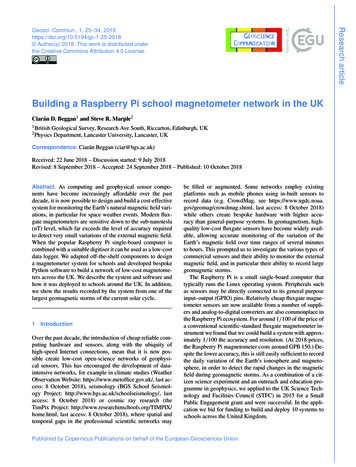
28C. Beggan and S. R. Marple: Raspberry Pi magnetometer networkFigure 1. Raspberry Pi magnetometer system: the computer and digitiser board are in the small box in the lower left corner (enclosed ina transparent plastic box). The sensor head contains three orthogonal fluxgate sensors in the Perspex cube, again contained in a transparentcase, which are connected by wires via the gray cable to the digitiser. A blue LED provides illumination to indicate the system is poweredon. The thermistor is located at the base of the sensor (not visible). Brass feet and a bubble spirit-level embedded in the base are used toensure the fluxgates are not tilted. The sensor head is approximately 15 cm high.ture, the magnetometer is also sensitive to man-made magnetic fields from mobile phones, vehicles or lifts in a building, for example. Consequently, we usually disregard the fullfield measurements and compute the variation of the horizontal field (H X2 Y 2 ) around a quiet-time value, usuallyconsidered to be around 02:00–03:00 LT (local time).We tested an initial prototype, placing it in an unused office at the British Geological Survey (BGS) building in Edinburgh, over several months in 2014 and compared its resultsto the data from the closest geomagnetic observatory in Eskdalemuir, Scotland. Figure 2 shows an example of 6 daysof data recorded on the Raspberry Pi magnetometer in Edinburgh. The horizontal strength (H ) was computed and theaverage value for the period was subtracted from the resultto give the variation. The blue line shows the data from theRaspberry Pi. For comparison, the data recorded on a scientific instrument (called Geomagnetic Data Acquisition System or GDAS1) at the Eskdalemuir Observatory approximately 70 km to the south of Edinburgh are shown in black.The data from the Edinburgh system closely match the variation recorded at the observatory.A number of different geomagnetic events were observed.On 12 September there was a geomagnetic storm whichGeosci. Commun., 1, 25–34, 2018caused the magnetic field to fluctuate from 125 to 125 nT.The storm ended on 13 September when the variations became smaller. The storm was followed by a series of smallerrapid wiggles (pulsations) which are the result of dissipation of energy from the magnetosphere. By 14 September,these disappeared and the ionospheric solar quiet-time (Sq)current became visible. This is seen as a daily fall and riseof about 20 nT, with its lowest point at noon when the Sunpasses overhead, on 15, 16 and 17 September. Finally, on17 September there is a step down and then up during theday time. This is man-made, caused by someone changingthe magnetic environment of the room (e.g. entering the roomfor a time and then leaving later in the day).Further testing of the second iteration of the sensor designwas carried out in late 2015. The updated magnetometer system was fitted with a solid-state temperature sensor and wasdeployed in Eskdalemuir for several weeks. It was placed in anon-temperature-controlled building around 100 m from theGDAS1 system. Figure 3a–b show the variation of the horizontal and vertical components compared to the EskdalemuirGDAS1 system. Panel (c) shows the difference between thetwo systems, with the temperature plotted too. There is astrong correlation between the magnetic differences of thewww.geosci-commun.net/1/25/2018/
C. Beggan and S. R. Marple: Raspberry Pi magnetometer network150100Geomagnetic stormPulsations50H [nT]29Daily Sq currentMan-made noise0 50Rpi horizontal (Edinburgh)GDAS1 horizontal (Eskdalemuir) 100 15012 Sep13 Sep14 Sep15 SepDate [2014]16 Sep17 Sep18 SepFigu
Jan 25, 2018 · The Raspberry Pi is a small single-board computer that typically runs the Linux operating system. Peripherals such as sensors may be directly connected to its general purpose input–output (GPIO) pins. Relatively cheap fluxgate magne-tometer sensors are now available from a number of