Transcription
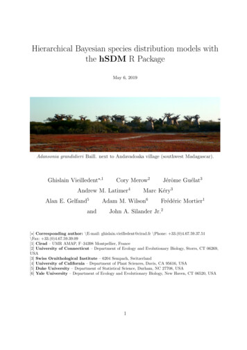
Species distribution modeling with RRobert J. Hijmans and Jane ElithJanuary 8, 2017
Chapter 1IntroductionThis document provides an introduction to species distribution modelingwith R . Species distribution modeling (SDM) is also known under other namesincluding climate envelope-modeling, habitat modeling, and (environmental orecological) niche-modeling. The aim of SDM is to estimate the similarity of theconditions at any site to the conditions at the locations of known occurrence(and perhaps of non-occurrence) of a phenomenon. A common application ofthis method is to predict species ranges with climate data as predictors.In SDM, the following steps are usually taken: (1) locations of occurrenceof a species (or other phenomenon) are compiled; (2) values of environmentalpredictor variables (such as climate) at these locations are extracted from spatialdatabases; (3) the environmental values are used to fit a model to estimatesimilarity to the sites of occurrence, or another measure such as abundance ofthe species; (4) The model is used to predict the variable of interest across anthe region of interest (and perhaps for a future or past climate).We assume that you are familiar with most of the concepts in SDM. If indoubt, you could consult, for example, Richard Pearson’s introduction to thesubject: sectionid 111, the book by Janet Franklin (2009), the somewhat more theoreticalbook by Peterson et al. (2011), or the recent review article by Elith and Leathwick (2009). It is important to have a good understanding of the interplay ofenvironmental (niche) and geographic (biotope) space – see Colwell and Rangel(2009) and Peterson et al. (2011) for a discussion. SDM is a widely used approach but there is much debate on when and how to best use this method.While we refer to some of these issues, in this document we do not provide anin-depth discussion of this scientific debate. Rather, our objective is to providepractical guidance to implemeting the basic steps of SDM. We leave it to youto use other sources to determine the appropriate methods for your research;and to use the ample opportunities provided by the R environment to improveexisting approaches and to develop new ones.We also assume that you are already somewhat familiar with the R languageand environment. It would be particularly useful if you already had some ex1
perience with statistical model fitting (e.g. the glm function) and with spatialdata handling as implemented in the packages ’raster’ and ’sp’. To familiarize yourself with model fitting see, for instance, the Documentation sectionon the CRAN webpage (http://cran.r-project.org/) and any introduction to Rtxt. For the ’raster’ package you could consult its vignette (available at ettes/Raster.pdf).When we present R code we will provide some explanation if we think it mightbe difficult or confusing. We will do more of this earlier on in this document,so if you are relatively inexperienced with R and would like to ease into it, readthis text in the presented order.SDM have been implemented in R in many different ways. Here we focuson the functions in the ’dismo’ and the ’raster’ packages (but we also referto other packages). If you want to test, or build on, some of the examplespresented here, make sure you have the latest versions of these packages, andtheir dependencies, installed. If you are using a recent version of R , you cando that with:install.packages(c(’raster’, ’rgdal’, ’dismo’, ’rJava’))This document consists of 4 main parts. Part I is concerned with data preparation. This is often the most time consuming part of a species distributionmodeling project. You need to collect a sufficient number of occurrence recordsthat document presence (and perhaps absence or abundance) of the species ofinterest. You also need to have accurate and relevant environmental data (predictor variables) at a sufficiently high spatial resolution. We first discuss someaspects of assembling and cleaning species records, followed by a discussion ofaspects of choosing and using the predictor variables. A particularly importantconcern in species distribution modeling is that the species occurrence data adequately represent the actual distribution of the species studied. For instance,the species should be correctly identified, the coordinates of the location dataneed to be accurate enough to allow the general species/environment to be established, and the sample unbiased, or accompanied by information on knownbiases such that these can be taken into account. Part II introduces the mainsteps in SDM: fitting a model, making a prediction, and evaluating the result.Part III introduces different modeling methods in more detail (profile methods,regression methods, machine learning methods, and geographic methods). InPart IV we discuss a number of applications (e.g. predicting the effect of climatechange), and a number of more advanced topics.This is a work in progress. Suggestions are welcomed.2
Part IData preparation3
Chapter 2Species occurrence dataImporting occurrence data into R is easy. But collecting, georeferencing, andcross-checking coordinate data is tedious. Discussions about species distributionmodeling often focus on comparing modeling methods, but if you are dealingwith species with few and uncertain records, your focus probably ought to beon improving the quality of the occurrence data (Lobo, 2008). All methodsdo better if your occurrence data is unbiased and free of error (Graham et al.,2007) and you have a relatively large number of records (Wisz et al., 2008).While we’ll show you some useful data preparation steps you can do in R ,it is necessary to use additional tools as well. For example, Quantum GIS,http://www.qgis.org/, is a very useful program for interactive editing of pointdata sets.2.1Importing occurrence dataIn most cases you will have a file with point locality data representing theknown distribution of a species. Below is an example of using read.table toread records that are stored in a text file. The R commands used are in italicsand preceded by a ’ ’. Comments are preceded by a hash (#). We are usingan example file that is installed with the ’dismo’ package, and for that reasonwe use a complex way to construct the filename, but you can replace that withyour own filename. (remember to use forward slashes in the path of filenames!).system.file inserts the file path to where dismo is installed. If you haven’tused the paste function before, it’s worth familiarizing yourself with it (type?paste in the command window). # loads the dismo librarylibrary(dismo)file - paste(system.file(package "dismo"), "/ex/bradypus.csv", sep "")# this is the file we will use:file4
[1] ypus.csv" # read itbradypus - read.table(file, header TRUE,# inspect the values of the file# first -65.3833-65.1333-63.6667-63.8500-64.4167sep .0000 # we only need columns 2 and 3: bradypus - bradypus[,2:3] 7.4500-17.4000-16.0000You can also read such data directly out of Excel files or from a database(see e.g. the RODBC package). Because this is a csv (comma separated values)file, we could also have used the read.csv function. No matter how you doit, the objective is to get a matrix (or a data.frame) with at least 2 columnsthat hold the coordinates of the locations where a species was observed. Coordinates are typically expressed as longitude and latitude (i.e. angular), butthey could also be Easting and Northing in UTM or another planar coordinatereference system (map projection). The convention used here is to organize thecoordinates columns so that longitude is the first and latitude the second column (think x and y axes in a plot; longitude is x, latitude is y); they often arein the reverse order, leading to undesired results. In many cases you will haveadditional columns, e.g., a column to indicate the species if you are modelingmultiple species; and a column to indicate whether this is a ’presence’ or an ’absence’ record (a much used convention is to code presence with a 1 and absencewith a 0).If you do not have any species distribution data you can get started by downloading data from the Global Biodiversity Inventory Facility (GBIF) (http://www.gbif.org/). In the dismo package there is a function ’gbif’ that youcan use for this. The data used below were downloaded (and saved to a permanent data set for use in this vignette) using the gbif function like this:5
acaule gbif("solanum", "acaule*", geo FALSE)If you want to understand the order of the arguments given here to gbif orfind out what other arguments you can use with this function, check out thehelp file (remember you can’t access help files if the library is not loaded), bytyping: ?gbif or help(gbif). Note the use of the asterix in ”acaule*” to notonly request Solanum acaule, but also variations such as the full name, Solanumacaule Bitter, or subspecies such as Solanum acaule subsp. aemulans.Many occurence records may not have geographic coordinates. In this case,out of the 1366 records that GBIF returned (January 2013), there were 1082records with coordinates (this was 699 and 54 in March 2010, a tremendousimprovement!) # load the saved S. acaule datadata(acaule)# how many rows and colums?dim(acaule)[1] 136625 #select the records that have longitude and latitude data ted""gbifNotes""maxElevationM""maxDepthM""ISO2" acgeo - subset(acaule, !is.na(lon) & !is.na(lat)) dim(acgeo)[1] 108225 # show some values acgeo[1:4, c(1:5,7:10)]12speciescontinentcountry adm1Solanum acaule Bitter South America Argentina JujuySolanum acaule Bitter South AmericaPeru Cusco6
3 Solanum acaule4 Solanum acauleadm21 Santa Catalina2Canchis3 NA 4 NA f. acaule NA Argentina NA f. acaule NA Bolivia NA latlon coordUncertaintyM alt-21.9000 -66.1000 NA NaN-13.5000 -71.0000 NA 4500-22.2666 -65.1333 NA 3800-18.6333 -66.9500 NA 3700Below is a simple way to make a map of the occurrence localities of Solanumacaule. It is important to make such maps to assure that the points are, at leastroughly, in the right location. library(maptools)data(wrld simpl)plot(wrld simpl, xlim c(-80,70), ylim c(-60,10), axes TRUE,col "light yellow")# restore the box around the mapbox()# plot pointspoints(acgeo lon, acgeo lat, col 'orange', pch 20, cex 0.75)# plot points again to add a border, for better visibilitypoints(acgeo lon, acgeo lat, col 'red', cex 0.75)7
The wrld simpl dataset contains rough country outlines. You can use otherdatasets of polygons (or lines or points) as well. For example, you can downloadhigher resolution data country and subnational administrative boundaries datawith the getData function of the raster package. You can also read your ownshapefile data into R using the shapefile function in the raster package.2.2Data cleaningData ’cleaning’ is particularly important for data sourced from species distribution data warehouses such as GBIF. Such efforts do not specifically gatherdata for the purpose of species distribution modeling, so you need to understandthe data and clean them appropriately, for your application. Here we providean example.Solanum acaule is a species that occurs in the higher parts of the Andesmountains of southern Peru, Bolivia and northern Argentina. Do you see anyerrors on the map?There are a few records that map in the ocean just south of Pakistan. Anyidea why that may have happened? It is a common mistake, missing minussigns. The coordinates are around (65.4, 23.4) but they should in NorthernArgentina, around (-65.4, -23.4) (you can use the ”click” function to query thecoordintates on the map). There are two records (rows 303 and 885) that map tothe same spot in Antarctica (-76.3, -76.3). The locality description says that isshould be in Huarochiri, near Lima, Peru. So the longitude is probably correct,and erroneously copied to the latitude. Interestingly the record occurs twice.The orignal source is the International Potato Center, and a copy is providedby ”SINGER” that aling the way appears to have ”corrected” the country toAntarctica: acaule[c(303,885),1:10]species continentcountry adm1303solanum acaule acaule NA Antarctica NA 885 solanum acaule acaule BITTER NA Peru NA adm2localitylatlon303 NA NA -76.3 -76.3885 NA Lima P. Huarochiri Pacomanta -76.3 -76.3coordUncertaintyM alt303 NA NaN885 NA 3800The point in Brazil (record acaule[98,]) should be in soutern Bolivia, so thisis probably due to a typo in the longitude. Likewise, there are also three recordsthat have plausible latitudes, but longitudes that are clearly wrong, as they arein the Atlantic Ocean, south of West Africa. It looks like they have a longitudethat is zero. In many data-bases you will find values that are ’zero’ where ’nodata’ was intended. The gbif function (when using the default arguments) sets8
coordinates that are (0, 0) to NA, but not if one of the coordinates is zero. Let’ssee if we find them by searching for records with longitudes of zero.Let’s have a look at these records: lonzero subset(acgeo, lon 0) # show all records, only the first 13 columns lonzero[, 164Solanum acauleSolanum acauleSolanum acauleSolanum acauleSolanum acauleSolanum acaulecountry adm1Argentina NA Bolivia NA Peru NA Peru NA Argentina NA Bolivia NA BitterBitterBitterBitterBitterBitteradm2 NA NA NA NA NA NA species continentsubsp. acaule NA subsp. acaule NA subsp. acaule NA subsp. acaule NA subsp. acaule NA subsp. acaule NA locality1159 between Quelbrada del Chorro and Laguna Colorada1160Llave1161km 205 between Puno and Cuzco1162km 205 between Puno and Cuzco1163 between Quelbrada del Chorro and Laguna Colorada1164Llavelat lon coordUncertaintyM alt institution1159 -23.7166670 NA 3400IPK1160 -16.0833340 NA 3900IPK1161 -6.9833330 NA 4250IPK1162 -6.9833330 NA 4250IPK1163 -23.7166670 NA 3400IPK1164 -16.0833340 NA 3900IPKcollection catalogNumber1159GBWKS 300271160GBWKS 300501161 WKS 300483047091162GBWKS 300481163 WKS 300273046881164 WKS 30050304711The records are from Bolivia, Peru and Argentina, confirming that coordinates are in error. Alternatively, it could have been that the coordinates werecorrect, perhaps referring to a location in the Atlantic Ocean where a fish was9
caught rather than a place where S. acaule was collected). Records with thewrong species name can be among the hardest to correct (e.g., distinguishingbetween brown bears and sasquatch, Lozier et al., 2009). The one record inEcuador is like that, there is some debate whether that is actually a specimenof S. albicans or an anomalous hexaploid variety of S. acaule.2.2.1Duplicate recordsInterestingly, another data quality issue is revealed above: each record in’lonzero’ occurs twice. This could happen because plant samples are often splitand send to multiple herbariums. But in this case it seems that the IPK (TheLeibniz Institute of Plant Genetics and Crop Plant Research) provided thesedata twice to the GBIF database (perhaps from seperate databases at IPK?).The function ’duplicated’ can sometimes be used to remove duplicates. # which records are duplicates (only for the first 10 columns)?dups - duplicated(lonzero[, 1:10])# remove duplicateslonzero - lonzero[dups, ]lonzero[,1:13]species continent1162 Solanum acaule Bitter subsp. acaule NA 1163 Solanum acaule Bitter subsp. acaule NA 1164 Solanum acaule Bitter subsp. acaule NA country adm1 adm21162Peru NA NA 1163 Argentina NA NA 1164Bolivia NA NA locality1162km 205 between Puno and Cuzco1163 between Quelbrada del Chorro and Laguna Colorada1164Llavelat lon coordUncertaintyM alt institution1162 -6.9833330 NA 4250IPK1163 -23.7166670 NA 3400IPK1164 -16.0833340 NA 3900IPKcollection catalogNumber1162GBWKS 300481163 WKS 300273046881164 WKS 30050304711Another approach might be to detect duplicates for the same species andsome coordinates in the data, even if the records were from collections by different people or in different years. (in our case, using species is redundant aswe have data for only one species)10
# differentiating by (sub) species# dups2 - duplicated(acgeo[, c('species', 'lon', 'lat')])# ignoring (sub) species and other naming variationdups2 - duplicated(acgeo[, c('lon', 'lat')])# number of duplicatessum(dups2)[1] 483 # keep the records that are not duplicated acg - acgeo[!dups2, ]Let’s repatriate the records near Pakistan to Argentina, and remove therecords in Brazil, Antarctica, and with longitude 0 i - acg lon 0 &acg lon[i] - -1 *acg lat[i] - -1 *acg - acg[acg lon2.3acg lat 0acg lon[i]acg lat[i] -50 & acg lat -50, ]Cross-checkingIt is important to cross-check coordinates by visual and other means. Oneapproach is to compare the country (and lower level administrative subdivisions) of the site as specified by the records, with the country implied by thecoordinates (Hijmans et al., 1999). In the example below we use the coordinates function from the sp package to create a SpatialPointsDataFrame, andthen the over function, also from sp, to do a point-in-polygon query with thecountries polygons.We can make a SpatialPointsDataFrame using the statistical function notation (with a tilde): library(sp)coordinates(acg) - lon latcrs(acg) - crs(wrld simpl)class(acg)[1] "SpatialPointsDataFrame"attr(,"package")[1] "sp"We can now use the coordinates to do a spatial query of the polygons inwrld simpl (a SpatialPolygonsDataFrame) class(wrld simpl)[1] "SpatialPolygonsDataFrame"attr(,"package")[1] "sp"11
ovr - over(acg, wrld simpl)Object ’ov’ has, for each point, the matching record from wrld simpl. Weneed the variable ’NAME’ in the data.frame of wrld simpl head(ovr)123456123456FIPS ISO2ARARPEPEARARBLBOBLBOBLBOSUBREGION555555ISO3 UNNAMEARG 32 ArgentinaPER 604PeruARG 32 ArgentinaBOL 68BoliviaBOL 68BoliviaBOL 68BoliviaLONLAT-65.167 -35.377-75.552 -9.326-65.167 -35.377-64.671 -16.715-64.671 -16.715-64.671 -16.715AREA POP2005 REGION273669 3874714819128000 2727426619273669 3874714819108438 918201519108438 918201519108438 918201519 cntr - ovr NAMEWe should ask these two questions: (1) Which points (identified by theirrecord numbers) do not match any country (that is, they are in an ocean)?(There are none (because we already removed the points that mapped in theocean)). (2) Which points have coordinates that are in a different country thanlisted in the ’country’ field of the gbif record i - which(is.na(cntr)) iinteger(0) j - which(cntr ! acg country) # for the mismatches, bind the country names of the polygons and points cbind(cntr, acg ""Argentina""Bolivia""Bolivia""Bolivia"In this case the mismatch is probably because wrld simpl is not very preciseas the records map to locations very close to the border between Bolivia and itsneighbors.12
plot(acg) plot(wrld simpl, add T, border 'blue', lwd 2) points(acg[j, ], col 'red', pch 20, cex 2)See the sp package for more information on the over function. The wrld simplpolygons that we used in the example above are not very precise, and theyprobably should not be used in a real analysis. See http://www.gadm.org/ formore detailed administrative division files, or use the ’getData’ function fromthe raster package (e.g. getData(’gadm’, country ’BOL’, level 0) to getthe national borders of Bolivia; and getData(’countries’) to get all countryboundaries).2.4GeoreferencingIf you have records with locality descriptions but no coordinates, you shouldconsider georeferencing these. Not all the records can be georeferenced. Sometimes even the country is unknown (country ”UNK”). Here we select onlyrecords that do not have coordinates, but that do have a locality description. georef - subset(acaule, (is.na(lon) is.na(lat)) & ! is.na(locality) ) dim(georef)[1] 1312513
georef[1:3,1:13]species continent country adm1606 solanum acaule acaule BITTER NA Bolivia NA 607 solanum acaule acaule BITTER NA Peru NA 618 solanum acaule acaule BITTER NA Peru NA adm2606 NA 607 NA 618 NA locality606 La Paz P. Franz Tamayo Viscachani 3 km from Huaylapuquio to Pelechuco607Puno P. San Roman Near Tinco Palca618Puno P. Lampa Saraccochalat lon coordUncertaintyM alt institution606 NA NA NA 4000PER001607 NA NA NA 4000PER001618 NA NA NA 4100PER001collection catalogNumber606 CIP - Potato collectionCIP-762165607 CIP - Potato collectionCIP-761962618 CIP - Potato collectionCIP-762376For georeferencing, you can try to use the dismo package function geocodethat sends requests to the Google API. We demonstrate below, but its use isgenerally not recommended because for accurate georeferencing you need a detailed map interface, and ideally one that allows you to capture the uncertaintyassociated with each georeference (Wieczorek et al., 2004).Here is an example for one of the records with longitude 0, using Google’sgeocoding service. We put the function into a ’try’ function, to assure eleganterror handling if the computer is not connected to the Internet. Note that weuse the ”cloc” (concatenated locality) field. georef cloc[4][1] "Ayacucho P. Huamanga Minas Ckucho, Peru" b - try(geocode(georef cloc[4]) )[1] "try 2 ."[1] "try 3 ."[1] "try 4 ." boriginalPlace interpretedPlace1 Ayacucho P. Huamanga Minas Ckucho, PeruNAlongitude latitude xmin xmax ymin ymax uncertainty1NANANANANANANA14
Before using the geocode function it is best to write the records to a tableand ”clean” them in a spreadsheet. Cleaning involves traslation, expandingabbreviations, correcting misspellings, and making duplicates exactly the sameso that they can be georeferenced only once. Then read the the table back intoR , and create unique localities, georeference these and merge them with theoriginal data.2.5Sampling biasSampling bias is frequently present in occurrence records (Hijmans et al.,2001). One can attempt to remove some of the bias by subsampling records,and this is illustrated below. However, subsampling reduces the number ofrecords, and it cannot correct the data for areas that have not been sampled atall. It also suffers from the problem that locally dense records might in fact bea true reflection of the relative suitable of habitat. As in many steps in SDM,you need to understand something about your data and species to implementthem well. See Phillips et al. (2009) for an approach with MaxEnt to deal withbias in occurrence records for a group of species. # create a RasterLayer with the extent of acgeor - raster(acg)# set the resolution of the cells to (for example) 1 degreeres(r) - 1# expand (extend) the extent of the RasterLayer a littler - extend(r, extent(r) 1)# sample:acsel - gridSample(acg, r, n 1)# to illustrate the method and show the resultp - rasterToPolygons(r)plot(p, border 'gray')points(acg)# selected points in redpoints(acsel, cex 1, col 'red', pch 'x')15
Note that with the gridSample function you can also do ’chess-board’ sampling. This can be useful to split the data in ’training’ and ’testing’ sets (seethe model evaluation chapter).At this point, it could be useful to save the cleaned data set. For examplewith the function write.table or write.csv so that we can use them later.We did that, and the saved file is available through dismo and can be retrievedlike this: file - paste(system.file(package "dismo"), '/ex/acaule.csv', sep '') acsel - read.csv(file)In a real research project you would want to spend much more time on thisfirst data-cleaning and completion step, partly with R , but also with otherprograms.2.6Exercises1) Use the gbif function to download records for the African elephant (or another species of your preference, try to get one with between 10 and 100records). Use option ”geo FALSE” to also get records with no (numerical) georeference.16
2) Summarize the data: how many records are there, how many have coordinates, how many records without coordinates have a textual georeference(locality description)?3) Use the ’geocode’ function to georeference up to 10 records without coordinates4) Make a simple map of all the records, using a color and symbol to distinguishbetween the coordinates from gbif and the ones returned by Google (viathe geocode function). Use ’gmap’ to create a basemap.5) Do you think the observations are a reasonable representation of the distribution (and ecological niche) of the species?More advanced:6) Use the ’rasterize’ function to create a raster of the number of observationsand make a map. Use ”wrld simpl” from the maptools package for country boundaries.7) Map the uncertainty associated with the georeferences. Some records in datareturned by gbif have that. You can also extract it from the data returnedby the geocode function.17
Chapter 3Absence and backgroundpointsSome of the early species distribution model algorithms, such as Bioclimand Domain only use ’presence’ data in the modeling process. Other methodsalso use ’absence’ data or ’background’ data. Logistic regression is the classicalapproach to analyzing presence and absence data (and it is still much used, oftenimplemented in a generalized linear modeling (GLM) framework). If you havea large dataset with presence/absence from a well designed survey, you shoulduse a method that can use these data (i.e. do not use a modeling method thatonly considers presence data). If you only have presence data, you can still use amethod that needs absence data, by substituting absence data with backgrounddata.Background data (e.g. Phillips et al. 2009) are not attempting to guess atabsence locations, but rather to characterize environments in the study region.In this sense, background is the same, irrespective of where the species has beenfound. Background data establishes the environmental domain of the study,whilst presence data should establish under which conditions a species is morelikely to be present than on average. A closely related but different concept,that of ”pseudo-absences”, is also used for generating the non-presence class forlogistic models. In this case, researchers sometimes try to guess where absencesmight occur – they may sample the whole region except at presence locations,or they might sample at places unlikely to be suitable for the species. We preferthe background concept because it requires fewer assumptions and has somecoherent statistical methods for dealing with the ”overlap” between presenceand background points (e.g. Ward et al. 2009; Phillips and Elith, 2011).Survey-absence data has value. In conjunction with presence records, itestablishes where surveys have been done, and the prevalence of the speciesgiven the survey effort. That information is lacking for presence-only data, afact that can cause substantial difficulties for modeling presence-only data well.However, absence data can also be biased and incomplete, as discussed in the18
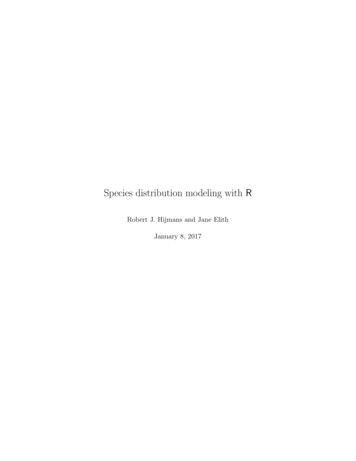
literature on detectability (e.g., Kéry et al., 2010).dismo has a function to sample random points (background data) from astudy area. You can use a ’mask’ to exclude area with no data NA, e.g. areas noton land. You can use an ’extent’ to further restrict the area from which randomlocations are drawn. In the example below, we first get the list of filenameswith the predictor raster data (discussed in detail in the next chapter). We usea raster as a ’mask’ in the randomPoints function such that the backgroundpoints are from the same geographic area, and only for places where there arevalues (land, in our case).Note that if the mask has the longitude/latitute coordinate reference system, function randomPoints selects cells according to cell area, which varies bylatitude (as in Elith et al., 2011) # get the file namesfiles - list.files(path paste(system.file(package "dismo"), '/ex',sep ''), pattern 'grd', full.names TRUE )# we use the first file to create a RasterLayermask - raster(files[1])# select 500 random points# set seed to assure that the examples will always# have the same random sample.set.seed(1963)bg - randomPoints(mask, 500 )And inspect the results by plotting # set up the plotting area for two mapspar(mfrow c(1,2))plot(!is.na(mask), legend FALSE)points(bg, cex 0.5)# now we repeat the sampling, but limit# the area of sampling using a spatial extente - extent(-80, -53, -39, -22)bg2 - randomPoints(mask, 50, ext e)plot(!is.na(mask), legend FALSE)plot(e, add TRUE, col 'red')points(bg2, cex 0.5)19
There are several approaches one could use to sample ’pseudo-absence’ points,i.e. points from more restricted area than ’background’. VanDerWal et al.(2009) sampled withn a radius of presence points. Here is one way to implement that, using the Solanum acaule data.We first read the cleaned and subsetted S. acaule data that we produced inthe previous chapter from the csv file that comes with dismo: file - paste(system.file(package "dismo"), '/ex/acaule.csv', sep '') ac - read.csv(file)ac is a data.frame. Let’s change it into a SpatialPointsDataFrame coordinates(ac) - lon lat projection(ac) - CRS(' proj longlat datum WGS84')We first create a ’circles’ model (see the chapter about geographic models),using an arbitrary radius of 50 km # circles with a radius of 50 km x - circl
Part III introduces di erent modeling methods in more detail (pro le methods, regression methods, machine learning methods, and geographic methods). In Part IV we discuss a number of applications (e.g. predicting the e ect of climate change), and a number of more advanced topics. This is a work in progress. Suggestions are welcomed. 2