Transcription
Revista Mexicana de Biodiversidad 79: 205- 216, 2008Modeling ecological niches and predicting geographic distributions: a test of sixpresence-only methodsModelado de nichos ecológicos y predicción de distribuciones geográficas: comparación de seismétodosMiguel A. Ortega-Huerta1 and A. Townsend Peterson21Instituto de Biología, Universidad Nacional Autónoma de México. Estación de Biología Chamela, Apartado postal 21, 48980, San Patricio, Jalisco,Mexico2Natural History Museum and Biodiversity Research Center, The University of Kansas, Lawrence, Kansas 66045 USA*Correspondent: maoh@ibiologia.unam.mxAbstract. Modeling ecological niches of species as a means to predict geographic distributions is a growing field thathas been applied to numerous challenges of importance in ecology, systematics, and human well-being. The increasingavailability and variety of such predictive algorithms requires testing their performance. In this study, we compare 6 suchalgorithms (Maxent, BioMapper, DOMAIN, FloraMap, the genetic algorithm GARP, and weights of evidence) as regardstheir ability to predict the geographic distributions of 10 species of Mexican birds for which ample distributional data areavailable. The results of this study nevertheless led to reflections on how model quality should be evaluated.Key words: ecological niche modeling, species’ distributions, algorithms, model validation.Resumen. La predicción de las distribuciones geográficas de las especies obtenida mediante el modelado de sus nichosecológicos, representa una línea de investigación en expansión, la cual ha sido aplicada en múltiples áreas de conocimientotales como ecología, sistemática y salud pública. La creciente disponibilidad y variedad de tales métodos y algoritmosde predicción determina su evaluación como necesaria. En este estudio, comparamos 6 algoritmos (Maxent, BioMapper,Domain, FloraMap, GARP, Weights of Evidence) con respecto a su habilidad para predecir las distribuciones geográficasde 10 especies de aves de México, para las cuales se cuenta con suficientes datos distribucionales. No obstante, losresultados de nuestro estudio sugieren la necesidad de elaborar nuevos criterios para la evaluación de modelos.Palabras clave: modelado de nichos ecológicos, distribuciones geográficas de especies, algoritmos, validación demodelos.IntroductionA growing field in ecology is that of modeling ecologicalniches for prediction of geographic distributions of species(Scott et al., 2002). These models permit analysis of a widevariety of biodiversity phenomena, including geographicdistributions (Elith and Burgman, 2002), future potentialdistributions under scenarios of climate change (Thomas etal., 2004), species’ invasions (Peterson, 2003), agriculturalcrop damage by pest organisms (Sánchez-Cordero andMartínez-Meyer, 2000), and priorities for biodiversityconservation (Chen and Peterson, 2002). Given theintense activity in this expanding field, the relative meritsof the various methods that have been employed to modelecological niches demand further exploration.Recibido: 29 enero 2007; aceptado: 12 noviembre 2007The methods that have been used for modelingecological niches are diverse, including multiple logisticregression and other forms of general linear models(Austin et al., 1990), set-based approaches characterizingranges of species along ecological dimensions (Nix, 1986),approaches based on distance measures in ecological space(Carpenter et al., 1993; Hirzel et al., 2002), maximumentropy approaches (Phillips et al., 2006), and geneticalgorithms (Stockwell, 1999; Stockwell and Noble, 1992;Stockwell and Peters, 1999), to name a few. Several studieshave developed comparisons among methods (Cumming,2000; Manel et al., 1999; Manel et al., 1999; Tsoar et al.,2007), but only one (Elith et al., 2006) has been at allcomprehensive, and many methods remain untested.A special focus has been on the use of presence-onlydata for modeling species distributions, even thoughthey face serious challenges in model inference relative
206Ortega-Huerta and Peterson.- Ecological niches and geographic distributionsto presence-absence methods (Wintle et al., 2005).Presence-only methods are necessary because absenceof species is difficult to demonstrate, and because falseabsences can decrease the reliability of predictive models(Chefaoui et al., 2005). A species may be recorded asabsent at a given location because the species is presentbut could not be detected, because the species is absentbut the habitat is suitable, or because the habitat is trulyunsuitable for the species, the former 2 situations canlead to identify false absences (Hirzel et al., 2002).Predicting species’ distributions from presence-only datasets and pseudoabsences (i.e., data resampled from areasnot holding presences) has the potential to be a usefulalternative when presence/absence data are unavailable orimpossible to obtain (Zaniewski et al., 2002; Brotons etal., 2004; Graham et al., 2004; Guisan and Thuiller, 2005).Among the attempts to evaluate presence-only models,Hirzel et al., (2006) identified 2 approaches: a), generatepseudoabsences and apply standard presence/absencetechniques, and b), assess how much model predictionsare better than random expectations.Because the challenges involved in modeling ecologicalniches may vary among regions and taxa, and given theintense efforts focused around understanding biodiversityphenomena in Mexico (CONABIO, 2002), this studywas developed to evaluate the behavior of 6 alternativemethodologies for Mexican taxa and landscapes. The6 methods were selected based in the different types ofalgorithms applied and the potential utility in modelingbiodiversity patterns. Three of the methodologies assessedhad not been compared with other approaches previously,even in the most comprehensive study to date (Elith et al.,2006).In this study, the models generated by each methodare analyzed as the ecological niche of 10 Mexican birdspecies for which ample distributional data are available.Our approach follows the relations between niche andspecies’ distribution proposed by Pulliam (2000): theGrinellian niche concept is that of the set of conditionssuitable to the point that the species can maintainpopulations. This study was neither designed to identify a‘best’ method, nor to make comparisons based on exactlythe same data. That is, each method was presented with aninformation base, and was allowed to use whatever portionof that information that it could; the relative merits of eachmethod are explored, and the behavior of each method ischaracterized. In particular, this investigation focused onreconsidering the methods by which we evaluate modelsto choose the ‘best’ ( most predictive) model, and on thequestion about the potential confusing role of statisticalsignificance as a measure of model’s predictive ability.Materials and methodsInput data. Comparisons among methods were based onstandard sets of information that were available to each. Foroccurrence information, we chose 10 bird species that 1),were well-sampled (N 100 unique occurrence points inMexico); 2), that showed a diversity of distributional areaswithin Mexico [e.g., from relatively restricted (Thryothorussinaloa) to relatively wide (Myadestes occidentalis)], and3), that varied in ecological requirements [e.g., desert(Campylorhynchus brunneicapillus), pine forest (Atlapetespileata), tropical forest (Tityra personata)]. In each case,we selected 50 unique occurrence points randomly, and setthem aside as an independent testing data set; models weredeveloped based on the remaining 50 occurrence pointsfor each species. (We used single random partitions onlyfor each species because of the computationally intensenature of several of the algorithms explored herein).Environmental data sets used in these modeling effortsincluded 10 raster GIS coverages with pixel resolution of0.05 . Themes included elevation, slope, and aspect (allresampled from 0.01 data sets available from the U.S.Geological Survey Hydro-1K digital elevation modeldataset, http://edcdaac.usgs.gov/gtopo30/hydro/; climatedata including annual mean, maximum, minimum,maximum daily, and minimum daily temperatures, andannual mean precipitation (from the Comisión Nacionalpara el Conocimiento y Uso de la Biodiversidad(CONABIO): http://www.conabio.gob.mx; and potentialvegetation (Rzedowski, 1978; also available from theCONABIO website). Different methods used most orall of these data layers, depending on their particularrequirements; however, one method, FloraMap, does notallow for user input of environmental data sets, and soused its own native climatic data only (Table 1). Details ofour implementation for each method follow.BioMapper. The ecological niche factor analysis (ENFA)implemented in BioMapper was developed by Hirzel et al.(2002) as a method to calculate habitat suitability mapswithout the need for data to document species’ absences.BioMapper is designed to compute factors that best explainspecies’ ecological distributions. Much as in principalcomponents analysis, factors extracted are by designuncorrelated, but in this case have biological significance.The first factor is the “marginality factor”,which describeshow far the species’ optimum conditions deviate from theconditions dominant in the study area. Next, “specializationfactors” are obtained that assess how the species’ variancediffers from the total variance in the ecological dimensions.Hence, in Biomapper, a relatively few factors explainmost of the variation in species’ ecological distributions.Main considerations in using Biomapper are as follows:
Revista Mexicana de Biodiversidad 79: 205- 216, 2008207Table 1. Environmental data coverages used by each algorithm in the development of ecological niche models fordistributional predictions. All coverages are continuous unless otherwise notedEnvironmental variablesBioMapperFloraMapDomainWeights ofevidenceGARPMaxentX(20 classes)X(20 classes)XXXXXElevationXXSlopeXXAspectAnnual mean temperatureMaximum temperatureMinimum temperatureMaximum daily temperatureMinimum daily temperatureAnnual mean precipitationXXXXXXXXXXXXXXPotential vegetation (categorical)XXXXXXXXMonthly rainfall (12 coverages)XMonthly average temperatures (12 coverages)XDiurnal temperature range (12monthly coverages)X1), the use of categorical variables in a factor analysisis puzzling, so potential vegetation was excluded fromanalyses; 2), data were normalized, applying the Box-Coxvariable transformation, and 3), habitat suitability mapswere generated (5 factors, 10 categories) via a series of1-dimensional histograms.Domain. Domain (Windows version 1.3) was implementedby the Center for International Forestry Research, Bogor,Indonesia, based on the original program (Carpenter et al.,1993). At its simplest, this algorithm generates maps ofecological similarity or distance (Gower metric) to thosesites at which the taxon is known to occur to predict thepotential geographic distribution of a species. For anylocation in the study area, Domain assigns each cell theGower distance between that cell and the closest point inthe training set. If averaging is enabled, the value stored isthe average of the n nearest cells. Analyses are generallyconducted with n 1, but larger values can be useful inreducing effects of outlier training points. Environmentalattributes were imported as continuous ASCII files with3 columns (longitude, latitude, value). Domain was usedapplying both complete categorical dissimilarity andcomplete similarity (1 - D) * 100. Weights of evidence.XXWeights of evidence is a quantitative method for combiningdata-based evidence in support of a hypothesis. The methodwas originally developed for non-spatial applications inmedical diagnosis, in which evidence consisted of a set ofsymptoms and the hypothesis was of the type “this patienthas disease X”. For each symptom, a pair of weightswas calculated, 1 for presence of the symptom, and 1 forabsence. The magnitude of the weights depended on theassociation measured between the symptom and the patternof disease in a large group of patients. These weights couldthen be used to estimate the probability that a new patientwould get the disease, based on the presence or absence ofsymptoms.Weights of evidence was adapted in the late 1980’sfor mapping mineral deposits with GIS (Raines et al.,2000), which is the implementation used herein. Here, theevidence consists of exploration data sets ( maps), and thehypothesis is “the location is favorable for occurrence ofdeposit type X”. Weights are estimated from the measuredassociation between known mineral occurrences and valueson the maps to be used as predictors. The hypothesis is thenevaluated repeatedly for the entire study area using thecalculated weights, producing a prediction of the species’
208Ortega-Huerta and Peterson.- Ecological niches and geographic distributionsdistribution in which evidence from several environmentalmap layers is combined. This technique belongs to a classof methods suitable for multi-criterion decision-making.Similar to multiple regression in statistics, this approachinvolves estimation of a response variable from a setof predictor variables based on Bayesian probabilities,with the assumption of conditional independence. Forimplementing this approach, it was necessary to definearea units in km2, so we re-projected all environmentallayers to a Lambert Conic Conformal projection.GARP. The Genetic Algorithm for Rule-set Predictionis a machine-learning meta-algorithm for ecologicalniche modeling and distributional prediction. Developedoriginally in UNIX (Stockwell, 1999; Stockwell andNoble, 1992; Stockwell and Peters, 1999), and now portedto Windows http://nhm.ku.edu/desktopgarp, GARP usesknown occurrence points and points resampled fromthe entire map to create populations of presences andpseudoabsences, respectively. Four simple subalgorithmsare used to create rules in the form of IF condition1 condition2 condition3 THEN prediction .These simple initial rules are then optimized via a geneticalgorithm, in which particular conditions may be perturbed,combined with conditions from other rules, etc. The endresult is a heterogeneous set of 20-50 rules, which inaggregate describe the ecological distribution of a species.In this implementation of GARP, we set the convergencecriterion to 0.01, and maximum iterations permitted to 1000.We ran 1000 models for each species, and selected the 10best (GARP models differ from one another owing to therandom-walk nature of the process) using a “best subsets”procedure that separates methods by their omissioncommission error characteristics (Anderson et al., 2003).MaxEnt. Maximum entropy is also a machine-learninggeneral-purpose method used to obtain predictions or makeinferences from incomplete information (Phillips et al.,2006). Given a set of samples (i.e., species occurrence) andset of features (environmental variables), MaxEnt estimatesniches by finding the distribution of probabilities closest touniform (maximum entropy), constrained to the fact thatfeature values match their empirical average (Phillips,2004). Phillips et al., (2006) document the main featuresof the MaxEnt software: 1), it uses presence-only data butcan also use presence-absence data; 2), environmental datamay be both continuous and categorical, and MaxEnt canincorporate interactions between variables; 3), efficientdeterministic algorithms make possible estimation of amaximum entropy probability distribution; 4), becauseof its mathematical definition, it is possible to interprethow environmental variables relate to model suitability;5), overfitting can be regulated, and 6), continuous outputmakes possible identification of fine distinctions of modelsuitability. The main disadvantage of MaxEnt is the needof further research into issues like regularization and theresults produced by the exponential probabilistic modelapplied.Even though MaxEnt performs internal modelvalidation tests, we decided to run this software using alltraining presence sites, evaluating model performanceoutside MaxEnt, as with the other methods. Mainparameters when running MaxEnt software included:feature types linear, quadratic, product, threshold, andhinge; regularization multiplier 3.0; regularization values(linear/quadratic/product 0.050, categorical 0.050,threshold 1.000, hinge 0.500): Maximum iterations 500, and convergence threshold 1.0 x g/ing/floramap101.htm) is based on calculations ofprobabilities that a particular climate condition belongs toa multivariate normal distribution at which a training setof occurrences has been found (Jones and Gladkov, 1999).The methodology may be extended to cover occurrencesof any organism with a distribution largely determined byclimate parameters.FloraMap uses a set of interpolated climate surfaces,a method for calculating the probability model, and amethod for mapping probabilities over the climate surface.Principal components analysis is used to construct setsof linear combinations of the raw climate variables thatmaximize the variance in each, are orthogonal to eachother, and are uncorrelated. In the end, each pixel ischaracterized in terms of distance to an n-dimensionalprobability density function.Our application of FloraMap used the FloraMapenvironmental data (per force). We used an 18 x 18 kmmap resolution, 31 variables in 3 groups (monthly rainfalltotals, monthly average temperatures, and monthlyaverage diurnal temperature range). We used power 0.50, with transformation [raina], and all weights set to1.0. The number of scores was set as N 7, and the lowestprobability 0.0005.Model evaluation. Two approaches were used to evaluatemodel performance—1 threshold-independent (ReceiverOperating Characteristics plots) and 1 threshold-dependent(chi-square tests)—each has strengths and weaknesses.The threshold-dependent approach is based on coincidencebetween test occurrence points and model predictions. A1-tailed chi-square test is built based on observed numbersof correct and incorrect predictions for the test occurrencepoints, in comparison with expected numbers derivedfrom product of the number of test occurrence points andthe proportional area predicted present versus absent. With1 degree of freedom, this approach provides an evaluationof how well the test occurrence points are predicted, taking
Revista Mexicana de Biodiversidad 79: 205- 216, 2008into account the proportional area predicted present. Whenmodel results are other than binary, however, a necessarystep is that of choosing a threshold above which theprediction is considered present. In this study, we chose athreshold for each species and method, based on the levelof prediction of the lowest prediction level for any of theinput (training) presence points (Pearson et al., 2006).For a threshold-independent evaluation of modelpredictivity, we used Receiver Operating Characteristic(ROC) analyses (Fielding and Bell, 1997). This statisticevaluates the sensitivity (absence of commission error)and specificity (absence of omission error) of a diagnostictest in the face of the independent testing dataset. Thetesting dataset provides a “gold standard” for presenceand an equal number of pixels from which the specieshas not been sampled (pseudoabsences) provide acharacterization of absence; each individual model isscored on its ability to predict the new data correctly.These scores are accumulated stepwise, and graphed onan axis of sensitivity (true positive rate of accumulation)and 1 - specificity (true negative rate of accumulation).The result is integrated to produce an area under the curve(AUC) that measures how well the model predicts the newpoint occurrences. The theoretically perfect result is AUC 1.0, whereas a test performing no better than randomyields AUC 0.5. The result can be evaluated using astandard normal approximation (z-test). All of our ROCanalyses were developed using SPSS statistical softwarev.13.0 (LEAD Technologies Inc.). Pseudoabsence datawere generated by selecting an equal population of points(N 50) randomly from those areas documented outsidethe known distributions of the species. Digital coveragesof the species documented geographic distributions wereobtained from the project NatureServe (Ridgely et al.,2005). A GIS software (ArcView 3.2) was used to isolatethe no-occurrence areas for each species and then togenerate 50 random sites within such areas.ResultsResults of the 6 approaches tested herein were variable,with predictions often ranging several-fold in area predictedpresent among methods for a given species (Fig. 1). Allapproaches agreed on what could be considered core areas(areas in which species are most likely to be found), inwhich test occurrence points had a high probability offalling.However, a spectrum of general tendencies could bedistinguished among the different algorithms, ranging from1), micro-prediction, in which only a core set of points wassuccessfully predicted; 2), generally good prediction, from209which small sets of points were nonetheless left out, and3), relatively broad predictions including areas larger thanthe distribution of the test occurrence points. Examples ofthese patterns can be seen in figure 1, in which weights ofevidence produces a micro-prediction, GARP produces arelatively large and inclusive prediction, and the remainingapproaches produce generally good predictions, but omitsome sets of points (Fig. 1, arrows).Testing these results across species and modelingapproaches using the threshold-dependent chi-squareapproach, almost all models for all species were seen tobe statistically significant (Table 2). Only 3 predictions(1 each for Weights of evidence, Domain, and MaxEnt)were not significantly better than a random prediction.As the chi-square statistic summarizes positive departurefrom random expectations, its magnitude can be used as anindex of model predictive ability (Peterson et al., 1999)—we noted that the average of the chi-square statistic acrossspecies was 79.1 for GARP, and lower (41.4-66.8) in theother methods, in spite of the broader areas predicted byGARP.The threshold-independent ROC approach showedsimilar trends (Figure 2): most predictions for most specieswere statistically significant (z-tests, P 0.05, Table 3).However, inspecting patterns of failures, FloraMap failedto achieve statistical significance in 2 of 10 species; andWeights of evidence in 1 species. The other 4 methodsproduced highly statistically significant predictions for allspecies.DiscussionThis analysis highlights several issues that challengethe growing field of modeling ecological niches andpredicting geographic distributions. In particular,questions revolve around issues such as spatial scale, userfriendliness, degree of customization necessary for analysisof a particular species, and computational demands. Someconjunction of these and other considerations will definethe ideal method, if 1 is to exist. We consider 2 suchquestions in detail below.Ability to use diverse environmental information. Onedimension in which we observed strong contrasts amongmethods was in the types of environmental informationthat could be used. At one end of the spectrum, FloraMapuses a predetermined set of 36 environmental variables,and does not admit any additional dimensions that auser might wish to include. Weights of evidence as acomputational algorithm clearly was near its limits (evenon reasonably fast CPUs) with the 10-dimension challengethat our analyses represented: not all of the climate layers
210Ortega-Huerta and Peterson.- Ecological niches and geographic distributionsFigure 1. Example results for the Golden-cheeked Woodpecker Melanerpes chrysogenys, across the 6 modeling approaches. Shadingramps are arbitrarily chosen, but with every effort to balance across methods. Arrows indicate failures of models to predict knownoccurrences.could be used, and those that were used had to be reclassed into 20 discrete, ordered categories. At the otherextreme, GARP and MaxEnt were able to use all of theenvironmental dimensions provided, including even apotential vegetation dataset that was categorical in nature;the other methods were not able to take advantage of thisdataset without further data transformations (e.g., usingBoolean maps in BioMapper). Hence, 2 of the methodsshowed significant limitations regarding ability to takeadvantage of numerous and diverse information sets.Model validation. The use of statistical significance as ameasure of model validity is generally accepted, and yetis worthy of some discussion (Fielding and Bell, 1997).Previous authors (Anderson et al., 2003) have arguedthat the “best” models may not be the most significantones; rather, best models should be identified basedon the specific combinations of Type I (omission) andType II (commission) errors that they present. It is worthnoting, for those who have dismissed the best-subsetsprocedure as a ‘GARP thing,’ that this approach can beused with deterministic algorithms if input occurrence orenvironmental data are manipulated using a bootstrap or
Revista Mexicana de Biodiversidad 79: 205- 216, 2008211Table 2. Summary of results of threshold-dependent chi-square tests of model quality for the 6 modeling methodsexamined. Obs correct number of points observed to be predicted successfully; Exp correct number of points expectedto be predicted successfully, given the area predicted present. Model failures are indicated in PBioMapperTyrannus crassirostrisMyadestes occidentalisTityra personataThryothorus sinaloaSittasomus griseicapillusOrtalis vetulaMitrephanes phaeocercusMelanerpes chrysogenysAtlapetes pileataCampylorhynchus .973.817.26.4 x 10-65.7 x 10-34.8 x 10-178.8 x 10-114.8 x 10-81.6 x 10-136.7 x 10-1010.0 x 10-158.8 x 10-183.4 x 10⁻⁵DomainTyrannus crassirostrisMyadestes occidentalisTityra personataThryothorus sinaloaSittasomus griseicapillusOrtalis vetulaMitrephanes phaeocercusMelanerpes chrysogenysAtlapetes pileataCampylorhynchus 15.026.729.43.0 x 10-90.1210.0 x 10-224.5 x 10-123.2 x 10-151.1 x 10-150.037.8 x 10-272.4 x 10-75.9 x 10-8FloraMapTyrannus crassirostrisMyadestes occidentalisTityra personataThryothorus sinaloaSittasomus griseicapillusOrtalis vetulaMitrephanes phaeocercusMelanerpes chrysogenysAtlapetes pileataCampylorhynchus 6168.170.47.23.4 x 10-132.9 x 10-63.0 x 10-197.8 x 10-214.5 x 10-161.8 x 10-141.5 x 10-132.0 x 10-384.8 x 10-177.3 x 10⁻³GARPTyrannus crassirostrisMyadestes occidentalisTityra personataThryothorus sinaloaSittasomus griseicapillusOrtalis vetulaMitrephanes phaeocercusMelanerpes chrysogenysAtlapetes pileataCampylorhynchus 1.395.251.920.47.5 x 10-248.8 x 10-132.8 x 10-306.4 x 10-203.3 x 10-213.1 x 10-181.2 x 10-211.8 x 10-225.9 x 10-136.3 x 10⁻⁶
212Ortega-Huerta and Peterson.- Ecological niches and geographic distributionsTable 2. ePMaxEntTyrannus crassirostrisMyadestes occidentalisTityra personataThryothorus sinaloaSittasomus griseicapillusOrtalis vetulaMitrephanes phaeocercusMelanerpes chrysogenysAtlapetes pileataCampylorhynchus .2176.6137.332.26.5 x 10-312.7 x 10-184.5 x 10-412.5 x 10-103.1 x 10-232.0 x 10-249.5 x 10-192.7 x 10-401.0 x 10-311.4 x 10-08Weights of evidenceTyrannus crassirostrisMyadestes occidentalisTityra personataThryothorus sinaloaSittasomus griseicapillusOrtalis vetulaMitrephanes phaeocercusMelanerpes chrysogenysAtlapetes pileataCampylorhynchus 30.847.597.522.21.8 x 10-151.4 x 10-172.1 x 10-251.8 x 10-123.1 x 10-271.5 x 10-180.385.6 x 10-125.4 x 10-232.5 x 10⁻⁶jackknife manipulation. Nonetheless, although developedfor replicate models from a single algorithm, this schemacan be a useful heuristic tool in the present comparisons(Anderson et al., 2003).The 2 significance tests used herein, however, bothbalance correct prediction of test points against proportionalarea predicted present. This balance, at first glance, isbeneficial: a “cheating” algorithm might simply predict theentire area present, and thus not fail in predicting presencefor a single point. However, with more careful inspection,this balance can distract from true predictivity (in thiscase, correct prediction of the entire range of distributionalpossibilities of a species). Consider the equation for thechi-square statistic, which is (O-E)2/E, where O and E areobserved and expected values, respectively. This number(and significance) can be maximized in 2 ways: eitherincrease the numerator ( correct prediction of test points)or decrease the denominator ( smaller area predicted).Particularly for species predicted to have wide-rangingdistributions (for which E is high), the latter can be mucheasier: micro-prediction of a subset of test points can bemore significant than more complete prediction of the testpoints. In this sense, these approaches have the potential toselect models that maximize the wrong quantity.Returning to the best-subsets comparison (Anderson etal., 2003), the best approaches to predicting distributionsof species would first and foremost minimize omission ofthe independent test points. Beyond that, their positionalong the commission axis (area predicted present) is lessclear—ce
absences can decrease the reliability of predictive models (Chefaoui et al., 2005). A species may be recorded as absent at a given location because the species is present but could not be detected, because the species is absent but the habitat is suitable, or because the habitat is truly unsuitable for the species, the former 2 situations can