Transcription
Hierarchical Bayesian species distribution models withthe hSDM R PackageMay 6, 2019Adansonia grandidieri Baill. next to Andavadoaka village (southwest Madagascar).Ghislain Vieilledent?,1Cory Merow2Andrew M. Latimer4Alan E. Gelfand5andJérôme Guélat3Marc Kéry3Adam M. Wilson6Frédéric Mortier1John A. Silander Jr.2[?] Corresponding author: \E-mail: ghislain.vieilledent@cirad.fr \Phone: 33.(0)4.67.59.37.51\Fax: 33.(0)4.67.59.39.09[1] Cirad – UMR AMAP, F–34398 Montpellier, France[2] University of Connecticut – Department of Ecology and Evolutionary Biology, Storrs, CT 06269,USA[3] Swiss Ornithological Institute – 6204 Sempach, Switzerland[4] University of California – Department of Plant Sciences, Davis, CA 95616, USA[5] Duke University – Department of Statistical Science, Durham, NC 27708, USA[6] Yale University – Department of Ecology and Evolutionary Biology, New Haven, CT 06520, USA1
2
Florebo quocumque ferar“I will flower everywhere I am planted”3
4
AbstractSpecies distribution models (SDM) are useful tools to explain or predict species range fromvarious environmental factors. SDM are thus widely used in conservation biology. Basedon the observations of the species in the field (occurence or abundance data), SDM facetwo major problems which lead to bias in models’ results: imperfect detection and spatialcorrelation of the observations.At the present time, there is a lack of statistical tools to analyse large occurence orabundance data-sets (typically with tens of hundreds observation points) taking into account both imperfect detection and spatial correlation.Here, we present the hSDM R package wich aims at providing user-friendly statistical functions to fill this gap. Functions were developped through a hierarchical Bayesianapproach. They call a Metropolis-within-Gibbs algorithm coded in C to estimate model’sparameters. Using compiled C code for the Gibbs sampler reduce drastically the computation time.By making these new statistical tools available to the scientific community, we hope todemocratize the use of more complex, but more realistic, statistical models for increasingknowledge in ecology and conserving biodiversity.Keywords: R, C code, site-occupancy models, CAR process, spatial autocorrelation, biodiversity, SDM, niche modelling, detection probability, counts data, presence-absence, false absence,uncertainty, hierachical Bayesian models, Metropolis, MCMC, Gibbs sampler5
6
CHAPTER1Introduction1.1Species distribution modelsBiogeography is the study of the distribution of species over space and time and biogeographers try to understand the factors determining a species distribution (Smith, 1868;Wallace, 1876). A species distribution is often represented with a map (Wallace, 1876).This knowledge on the ecology of the species can be used for several applications such asconservation biology (Thuiller, 2014).Species distribution modelling (alternatively known as “environmental niche modelling”,“ecological niche modelling”, “predictive habitat distribution modelling”, and “climate envelope modelling”) refers to the process of using computer algorithms to predict the distribution of species in geographic space on the basis of a mathematical representation oftheir known distribution in environmental space (i.e. the realized ecological niche). Theenvironment is in most cases represented by climate data (such as temperature, and precipitation), but other variables such as soil type and land cover can also be used. Speciesdistribution models (SDM) allow estimating the probability of presence or abundance of aspecies on a large geographical range using a limited number of species observations (Elith& Leathwick, 2009; Guisan & Zimmermann, 2000). Species observations can be occurencedata (presence-absence data or presence only data) or abundance data (also known ascount data).7
1.2Imperfect detection and spatial correlation of theobservationsWhen considering presence-absence or abundance data for species distribution modelling,strong assumptions are usually made (Araujo & Guisan, 2006; Guisan & Thuiller, 2005;Sinclair et al., 2010). Among these assumptions, two can lead to biased estimates of speciesdistribution. The first one deals with imperfect detection and the second one with spatialcorrelation of the observations.Regarding imperfect detection, occurrence of a species is typically not observed perfectly. Species traits, survey-specific conditions and site-specific characteristics may influence species detection probability which is often 1 (Chen et al., 2013). Thus, observationsmight include false absences. For example, the habitat can be suitable and the species ispresent but individuals have not been seen during the census. Or the habitat can be suitable but the species has not dispersed yet to the site (typical example for plant species,see Latimer et al. (2006)) or was not present on the site at the moment of the observation(typical example for animal species such as birds, see Kéry et al. (2005)). Treating observedoccurrence and species distributions as the true occurrence and distribution, failing to makeamendments for imperfect detection, may lead to problems in species distribution studies, habitat models and biodiversity management (Kéry & Schmidt, 2008; Lahoz-Monfortet al., 2014; Latimer et al., 2006).Regarding spatial correlation, most species present geographical patchiness (positivespatial autocorrelation). This pattern is often driven by multiple causes that may be associated to exogenous environmental factors such as climate or soil (which might be partlytaken into account in species distribution models), but also to endogeneous biotic processes, called contagious processes, such as dispersal, migration, conspecific attraction ormortality which are rarely considered (Dormann et al., 2007; Legendre, 1993; Lichsteinet al., 2002; Sokal & Oden, 1978). Due to the contagious biotic processes, the presence orabundance of a species at one site is influenced by the presence or abundance of the speciesat surrounding sites. A species might be present at a site where the environment is lesssuitable because of the presence of the species at neighbouring sites where the environmentis higly suitable. Thus, ignoring spatial correlation may lead to biased conclusions aboutecological relationships (Lichstein et al., 2002) and even invert the slope of relationshipsfrom non-spatial analysis in some particular cases (Kühn et al., 2006). In addition toits ecological significance, spatial autocorrelation is problematic for classical species distribution models which assume independently distributed errors (Dormann et al., 2007;Legendre, 1993; Lichstein et al., 2002).8
1.3Methods and software to account for imperfectdetection and spatial correlationNew classes of models, called site-occupancy models (MacKenzie et al., 2002) or zeroinflated binomial (ZIB) models (Latimer et al., 2006) for presence-absence data and Nmixture models (Royle, 2004) or zero inflated Poisson (ZIP) models for abundance data(Flores et al., 2009), were developed to solve the problems created by imperfect detection.These models combine two processes, an ecological process which describes habitat suitability and an observation process which takes into account imperfect detection. Becausethey mix probability distributions to represent the suitability and observation processes,these models have also been called mixture models. Mixture models use information fromrepeated observations at several sites to estimate detectability. Detectability may varywith site characteristics (e.g., habitat variables) or survey characteristics (e.g., weatherconditions), whereas suitability relates only to site characteristics.One additional point regarding site-occupancy models is that they form a unifyingframework for a very large array of capture-recapture models to estimate population size inanimal ecology (Nichols, 1992): using parameter-expanded data augmentation (Royle et al.,2007), most models for population size, survival, recruitment and similar demographicquantities (presented in detail in standard references such as Williams et al. (2002), Royle &Dorazio (2008) and Kéry & Schaub (2012)) can be cast into the framework of an occupancymodel and this makes their fitting much easier.Several studies have demonstrated the advantages of site-occupancy and N-mixturemodels over classical models which do not consider imperfect detection. These studieshave focused on the distribution of various plant or animal species in marine and terrestrialecosystems (see Chen et al. (2013); Latimer et al. (2006) for plants, Dorazio et al. (2006);Kéry et al. (2005); Rota et al. (2011); Royle (2004) for birds, Kéry et al. (2010) for insects,Bailey et al. (2004); Chelgren et al. (2011); MacKenzie et al. (2002) for amphibians, Monk(2014) for fishes, and Gray (2012); Poley et al. (2014) for mammals).Several softwares can be used to fit site-occupancy and N-mixture models (Table 1.2).Some are based on the maximum likelihood approach (such as the widely used free Windowsprograms MARK and PRESENCE and the R package unmarked) while other are basedon the hierarchical Bayesian approach (such as WinBUGS and OpenBUGS programs).9
ross-platformcross-platformMS-WBayesian cross-platformBayesian entTeam (2014)Lunn et al.(2009)Lunn et al.(2009)MacKenzie(2006)White &Burnham (1999)Choquet et al.(2009)Fiske &Chandler (2011)Johnson et unmarkedE-SURGEMARKPRESENCEURLTable 1.2: Softwares available for modeling species distribution including imperfect 111MARKJAGSStan1SoccPRESENCESoftwares
A variety of methods have been developed to correct for the effects of spatial autocorrelation in species distribution models based on occurence or abundance data (Cressie &Cassie, 1993; Dormann et al., 2007; Keitt et al., 2002; Miller et al., 2007). In their reviewarticle, Dormann et al. (2007) described six different statistical approaches to account forspatial autocorrelation: autocovariate regression; spatial eigenvector mapping; generalisedleast squares; autoregressive models and generalised estimating equations.Several studies have demonstrated the advantages of these mehods focusing on a varietyof plant or animal species (see Gelfand et al. (2005); Kühn et al. (2006); Latimer et al.(2006) for plants, Lichstein et al. (2002) for birds, and Johnson et al. (2013); Poley et al.(2014) for mammals).Among the methods available to account for spatial autocorrelation, conditional autoregressive (CAR) models, which incorporate spatial autocorrelation through a neighbourhood structure, are commonly implemented in statistical softwares (Dormann et al.,2007). The most commonly used softwares to implement CAR models are OpenBUGSand WinBUGS softwares (Lunn et al., 2009) which have in-built functions (car.normaland car.proper) to describe the CAR process. CAR models can also be implementedin BayesX (Brezger et al., 2005) and in the following R packages: R-INLA (Rue et al.,2009), CARBayes (Lee, 2013), stocc (for binary data only), spatcounts (for count dataonly), CARramps (for Gaussian data only), and spdep (for Gaussian data only) (Table 1.4).11
Bayesian cross-platformBayesian cross-platformML cross-platformBayesian cross-platformBayesian cross-platformBayesian oachLunn et al.(2009)Lunn et al.(2009)Brezger et al.(2005)Rue et al.(2009)Lee (2013)Johnson et yesstoccR-INLABayesXWinBUGSOpenBUGSURLTable 1.4: Softwares available for modeling species distribution including spatial autocorrelation.countGaussianGaussianbinomial and allallallWinBUGSCARBayesstoccallType of dataOpenBUGSSoftwares
1.4Objectives of the hSDM R packageAmong the available statistical programs, only OpenBUGS can be used on any operatingsystem to fit both site-occupancy or N-mixture models including also a spatial autocorrelation process (Table 1.2 and Table 1.4). One problem is that OpenBUGS, for suchmodels, cannot handle large data-sets (typically, data-sets with tens of thousands sites).Moreover, for smaller data-sets, models can be fitted but computation time can be long dueto the fact that the OpenBUGS code is interpreted and not compiled. For this reason,we decided to develop the hSDM (for hierarchical Bayesian species distribution models) Rpackage. The stocc R package (Johnson et al., 2013; Poley et al., 2014), which can handlebinary data only, has been developed for the same reasons. The hSDM package allowsthe user to fit mixture models which take into account imperfect detection (site-occupancy,N-mixture, ZIB and ZIP models) and account for spatial autocorrelation. Spatial autocorrelation is represented through an intrinsic CAR process (Besag et al., 1991). Functionsin the hSDM R package use an adaptive Metropolis algorithm (Metropolis et al., 1953;Robert & Casella, 2004) in a Gibbs sampler (Casella & George, 1992; Gelfand & Smith,1990) to obtain the posterior distribution of model’s parameters. The Gibbs sampler iswritten in C code and compiled to optimize computation efficiency. Thus, the hSDMpackage can be used for very large data-sets while reducing drastically the computationtime.In this vignette, we present examples to illustrate the use of the hSDM package in theR statistical environment (R Development Core Team, 2014). Examples use virtual or realdata-sets. Results obtained with functions in the hSDM package are compared with theresults obtained with other softwares and models.13
14
CHAPTER2Occurence data2.12.1.1Binomial modelMathematical formulationLet’s consider a random variable yi representing the total number of presences of a speciesafter several visits vi at a particular site i. Random variable yi can take values from 0to vi and can be assumed to follow a Binomial distribution having parameters vi and θi(Eq. 2.1). Parameter θi can be interpreted as the probability of presence of the speciesat site i . Using a logit link function, θi can be expressed as a linear model combiningexplicative variables Xi and parameters β (Eq. 2.1).yi Binomial(vi , θi )(2.1)logit(θi ) Xi βUsing this statistical model, we aim at representing a “suitability process”. Givenenvironmental variables Xi , how much is habitat at site i suitable for the species underconsideration? Parameters β indicate how much each environmental variable contributesto the suitability process. Like every other function in the hSDM R package, functionhSDM.binomial() estimates the parameters β of such a model in a Bayesian framework.Parameter inference is done using a Gibbs sampler including a Metropolis algorithm. TheGibbs sampler is coded in the C language to optimize computation efficiency.15
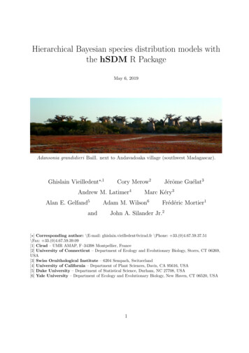
2.1.2Data generationTo explore the characteristics of the hSDM.binomial() function, we generate a virtualdata-set on the basis of the Binomial model described above (Eq. 2.1). In the most generalcase, sites are visited once (vi 1). Thus, the random variable yi follows a Bernoullidistribution of parameter θi and habitat characteristics Xi are fixed for site i. We generatea virtual data-set in this particular case. For data generation, we import virtual altitudinaldata in R. Altitude is used as an explicative variable to determine habitat suitability, i.e.the probability of presence of a virtual species. Altitudinal data are loaded at the sametime as the hSDM R package (data frame altitude in the working directory).These data are transformed into a raster object using the function rasterFromXYZ()from the raster package. The raster has 2500 cells (50 columns and 50 rows) and thealtitude ranges roughly between 100 and 600 m (Fig. 2.1). For linear models, explicativevariables are usually centered and scaled to facilitate inference and interpretation of modelparameters.# Load altitudinal data and create ckage "hSDM")alt.orig - rasterFromXYZ(altitude)extent(alt.orig) - c(0,50,0,50)plot(alt.orig)# Center and scale altitudinal dataalt - scale(alt.orig,center TRUE,scale TRUE)plot(alt)A linear model including altitude (variable denoted A) is used to compute the probability of presence of the species (Eq. 2.2).yi Bernoulli(θi )(2.2)logit(θi ) β0 β1 AiWe fix the parameters to β0 1 and β1 1. The species has a higher probability ofpresence at higher altitudes (Fig. 2.2).# Target parametersbeta.target - matrix(c(-1,1),ncol 1)# Matrix of covariates (including the intercept)ncells - ncell(alt)X - cbind(rep(1,ncells),values(alt))# Probability of presence as a linear function of altitudelogit.theta - X %*% beta.target16
50405040130305000400 12020300 2200100010 30102030405001020304050Figure 2.1: Altitudinal data. Original values (in m) on the left. Centered and scaledvalues on the right.theta - inv.logit(logit.theta)# Coordinates of raster cellscoords - coordinates(alt)# Transform the probability of presence into a rastertheta - rasterFromXYZ(cbind(coords,theta))# Color palette for probability plotscolRP - ,"brown","black"))# Plot the probability of presencebrks - seq(0,1,length.out 100)arg - list(at seq(0,1,length.out 5), labels c("0","0.25","0.5","0.75","1"))nb - length(brks)-1plot(theta,main "Initial probabilities",col colRP(nb),breaks brks,axis.args arg,zlim c(0,1))We can assume a number n of sites in the landscape where we have been able to observeor not the presence of the species. We can simulate the presence or absence of the speciesat these n sites given our model (Fig. 2.3).# Number of observation sitesnsite - 200# Set seed for repeatabilityseed - 1234# Sample the observations in the landscape17
4050Initial probabilities1300.75200.50.25010001020304050Figure 2.2: Probability of presence.set.seed(seed)x.coord - runif(nsite,0,50)set.seed(2*seed)y.coord - runif(nsite,0,50)library(sp)sites.sp - SpatialPoints(coords cbind(x.coord,y.coord))# Extract altitude data for sitesalt.sites - extract(alt,sites.sp)# Compute theta for these observationsX.sites - cbind(rep(1,nsite),alt.sites)logit.theta.site - X.sites %*% beta.targettheta.site - inv.logit(logit.theta.site)# Simulate observationsvisits - rep(1,nsite) # One visit per site for the momentset.seed(seed)Y - rbinom(nsite,visits,theta.site)# Group explicative and response variables in a data-framedata.obs.df - data.frame(Y,visits,alt X.sites[,2])# Transform observations in a spatial objectdata.obs - SpatialPointsDataFrame(coords coordinates(sites.sp),data data.obs.df)# Plot observationsplot(alt.orig)points(data.obs[data.obs Y 1,],pch 16)points(data.obs[data.obs Y 0,],pch 1)18
50 40 20 10 200 0 4050 10 300 400 0 500 30 2030Figure 2.3: Observation points. Presences (full circles) and absences (empty circles) arelocalized on the altitude map (in m).2.1.3Parameter inference using the hSDM.binomial() functionThe hSDM.binomial() function performs a Binomial logistic regression in a Bayesianframework. Before using this function we need to prepare a bit the data for predictions.We want to have predictions on the whole landscape, not only at observation points. Todirectly obtain these predictions, we can create a data frame including altitudinal data onthe whole landscape. This data frame will be used for the suitability.pred argument.The data frame for predictions must include the same column names as those used in theformula for the suitability argument (i.e. “alt” our example).data.pred - data.frame(alt values(alt))We can now call the hSDM.binomial() function. Setting parameter save.p to 1, we cansave in memory the MCMC values for predictions. These values can be used to computeseveral statistics for each predictions (mean, median, 95% quantiles). For example, meanand 95% quantiles are useful to estimate the uncertainty around the mean predictions.mod.hSDM.binomial - hSDM.binomial(presences data.obs Y,trials data.obs visits,suitability alt,19
data data.obs,suitability.pred data.pred,burnin 1000, mcmc 1000, thin 1,beta.start 0,mubeta 0, Vbeta 1.0E6,seed 1234, verbose 1, save.p 1)2.1.4Analysis of the resultsThe hSDM.binomial() function returns an MCMC (Markov chain Monte Carlo) for eachparameter of the model and also for the model deviance. To obtain parameter estimates,MCMC values can be summarized through a call to the summary() function from the codapackage. We can check that the values of the target parameters, β0 1 and β1 1, arewithin the 95% confidence interval of the parameter estimates.summary(mod.hSDM.binomial tions 1001:2000Thinning interval 1Number of chains 1Sample size per chain 10001. Empirical mean and standard deviation for each variable,plus standard error of the mean:MeanSD Naive SE Time-series SEbeta.(Intercept) -1.4127 0.2255 0.0071310.02234beta.alt0.9844 0.2961 0.0093630.03277Deviance202.1663 2.2848 0.0722520.166072. Quantiles for each variable:2.5%25%50%75%97.5%beta.(Intercept) -1.8432 -1.5566 -1.4128 -1.265 ce199.8948 200.4900 201.3279 203.193 207.6644Parameters estimates can be compared to results obtained with the glm() function.# glm results for comparisonmod.glm - glm(cbind(Y,visits-Y) alt,family "binomial",data data.obs)summary(mod.glm)20
:glm(formula cbind(Y, visits - Y) alt, family "binomial",data data.obs)Deviance Residuals:Min1QMedian-1.1290 -0.7509 -0.60413Q-0.1749Max2.7277Coefficients:Estimate Std. Error z value(Intercept) -1.38220.1966 -7.032alt0.95180.27643.444--Signif. codes: 0 '***' 0.001 '**' 0.01Pr( z )2.03e-12 ***0.000573 ***'*' 0.05 '.' 0.1 ' ' 1(Dispersion parameter for binomial family taken to be 1)Null deviance: 215.71Residual deviance: 199.79AIC: 203.79on 199on 198degrees of freedomdegrees of freedomNumber of Fisher Scoring iterations: 5MCMC can also be graphically summarized with a call to the plot.mcmc() function,also in the coda package. MCMC are plotted with a trace of the sampled output and adensity estimate for each variable in the chain (Fig. 2.4). This plot can be used to visuallycheck that the chains have converged.plot(mod.hSDM.binomial mcmc)The hSDM.binomial() function also returns two other objects. The first one, theta.latent,is the predictive posterior mean of the latent variable θ (the probability of presence) foreach observation.str(mod.hSDM.binomial theta.latent)##num [1:200] 0.2191 0.0992 0.1038 0.1878 0.221 .summary(mod.hSDM.binomial theta.latent)####Min. 1st Qu.0.0171 0.1540Median0.2179Mean 3rd Qu.0.2297 0.297421Max.0.4970
Density of beta.(Intercept)0.00.51.01.5 2.0 1.6 1.2 0.8Trace of beta.(Intercept)12001400160018002000 2.0 1.5 1.0IterationsN 1000 Bandwidth 0.05789Trace of beta.altDensity of 0000.00.51.01.5IterationsN 1000 Bandwidth 0.0779Trace of DevianceDensity of 01400160018002000200Iterations205210215N 1000 Bandwidth 0.5371Figure 2.4: Trace and density estimate for each variable of the MCMC.22
The second one, theta.pred is the set of sampled values from the predictive posterior(if parameter save.p is set to 1) or the predictive posterior mean (if save.p is set to 0)for each prediction. In our example, save.p is set to 1 and theta.pred is an mcmc object.Values in theta.pred can be used to plot the predicted probability of presence on thewhole landscape and the uncertainty associated to predictions (Fig 2.5).# Create a raster for predictionstheta.pred.mean - raster(theta)# Create rasters for uncertaintytheta.pred.2.5 - theta.pred.97.5 - raster(theta)# Attribute predicted values to raster cellstheta.pred.mean[] - apply(mod.hSDM.binomial theta.pred,2,mean)theta.pred.2.5[] - apply(mod.hSDM.binomial theta.pred,2,quantile,0.025)theta.pred.97.5[] - apply(mod.hSDM.binomial theta.pred,2,quantile,0.975)# Plot the predicted probability of presence and uncertaintyplot(theta.pred.mean,main "Mean",col colRP(nb),breaks brks,axis.args arg,zlim c(0,1))plot(theta.pred.2.5,main "Quantile 2.5 %",col colRP(nb),breaks brks,axis.args arg,zlim c(0,1))plot(theta.pred.97.5,main "Quantile 97.5 %",col colRP(nb),breaks brks,axis.args arg,zlim c(0,1))In our example, we can compare the predictions to the initial probability of presencecomputed from our model to check that our predictions are correct (Fig. 2.6).# Comparing predictions to initial valuesplot(theta[],theta.pred.mean[],cex.lab 1.4,xlim c(0,1),ylim c(0,1))points(theta[],theta.pred.2.5[],cex.lab 1.4,col grey(0.5))points(theta[],theta.pred.97.5[],cex.lab 1.4,col grey(0.5))abline(a 0,b 1,col "red",lwd 2)23
530304050Quantile 97.5 %50Quantile 2.5 igure 2.5: Predicted probability of presence and uncertainty of predictions.Mean probability of presence (top), predictions at 2.5% quantile (bottom left) and 97.5%quantile (bottom right) can be plotted from the mcmc object plot.p.pred returned byfunction hSDM.binomial().24
1.00.80.60.4theta.pred.mean[]0.20.0 0.00.20.40.60.81.0theta[]Figure 2.6: Predicted vs. initial probabilities of presence. Initial probabilities ofpresence are computed from the Binomial logistic regression model with target parameters.2.22.2.1Site-occupancy modelMathematical formulationLet’s consider the random variable zi describing habitat suitability at site i. The randomvariable zi can take value 1 or 0 depending on the fact that the habitat is suitable (zi 1)or not (zi 0). Habitat at site i is described by environmental variables Xi . Randomvariable zi can be assumed to follow a Bernoulli distribution of parameter θi (Eq. 2.3). Inthis case, θi is the probability that the habitat is suitable. Several visits at time t1 , t2 ,etc., can occur at site i. Let’s consider the random variable yit representingthe presencePof the species at site i and time t. The species is observed at site i ( Pt yit 1) only ifthe habitat is suitable (zi 1). The species is unobserved at site i ( t yit 0) if thehabitat is not suitable (zi 0), or if the habitat is suitable (zi 1) but the probabilityδit of detecting the species at site i and time t is inferior to 1. Thus, yit is assumed tofollow a Bernoulli distribution of parameter zi δit . Using a logit link function, δit can beexpressed as a linear model combining explicative variables Wit and parameters γ (Eq. 2.3).Typically, explicative variables Wit are site characteristics (e.g., habitat variables) or surveycharacteristics (e.g., weather conditions). The function hSDM.siteocc() estimates theparameters β and γ of such a model.25
Ecological process:zi Bernoulli(θi )logit(θi ) Xi β(2.3)Observation process:yit Bernoulli(zi δit )logit(δit ) Wit γ2.2.2Data generationTo explore the characteristics of the hSDM.siteocc() function, we can generate a newvirtual data-set on the basis of the site-occupancy model described above (Eq. 2.3). Inthe most general case, the observation protocol includes severals visits with varying surveyconditions (e.g. weather conditions) to several sites with fixed sites characteristics (e.g.habitat variables). We will generate a virtual data-set following this protocole using thealtitudinal data in the previous example for the Binomial model (Sec. 2.1).We draw at random the number of visits at each site of the previous example (seeFig. 2.3 of Sec. 2.1).# Number of visits associated to each observation pointset.seed(seed)visits - rpois(nsite,lambda 3) # Mean number of visits 3# NB: Setting a too low mean number of visits per site (lambda 3)# leads to inaccurate parameter estimatesvisits[visits 0] - 1 # Number of visits must be 0# Vector of observation sitessites - vector()for (i in 1:nsite) {sites - c(sites,rep(i,visits[i]))}The survey conditions for each visit are determined by two explicative variables, w1and the altitude (variable denoted A). These two variables explain the observability of thespecies (Eq. 2.4).(2.4)yit Bernoulli(zi δit )logit(δit ) γ0 γ1 w1it γ2 AitWe fix the intercept and the effects of these two variables: γ0 1, γ1 1 and γ2 1for determining the detection probability. In our case, the detection probability decreaseswith altitude (γ2 0).26
# Explicative variables for observation processnobs - sum(visits)set.seed(seed)w1 - rnorm(n nobs,0,1)W - cbind(rep(1,nobs),w1,X.sites[sites,2])# Target parameters for observation processgamm
CHAPTER 1 Introduction 1.1 Species distribution models Biogeography is the study of the distribution of species over space and time and biogeog-raphers try to understand the factors determining a species distribution (Smith,1868;