WIXLIB

2012 Conference on Intelligent Data UnderstandingWe used several decision trees in our experiments. Adecision tree is a tree in which each branch node represents achoice between a number of alternative properties, whereineach leaf node represents a classification or decision. Theimportant function to consider when building a decision treeis known as the splitting criterion, which defines how datashould be split in order to maximize performance.C4.5 builds decision trees from a set of training data usingthe concept of information entropy, a measure of uncertainty,to define the splitting criteria [17].CART uses the Gini index, a measure of how often arandomly chosen element from the set would be incorrectlylabeled if it were randomly labeled according to the distribution of labels in the subset [1]. While C4.5 and CARTcan be effective on datasets that have been sampled, theyare considered to be “skew sensitive” [10]; that is, themethods can become biased as the degree of class imbalanceincreases.HDDT, another decision tree, uses the measure ofHellinger distance to decide between alternative properties,a measure that quantifies the similarity between two probability distributions [4][19]. By using this measure, HDDTcapitalizes on the importance of designing a decision treesplitting criterion that captures the divergence in distributions while being skew-insensitive [5].Random Forest is an ensemble classifier that consists ofmany decision trees and outputs the class that is the mode ofthe classes output by individual trees [2]. In our experiments,we ran two implementations of Random Forest: one simplyused Random Forest with the generated training sets, theother used Random Forest with SMOTE applied to thetraining sets.SMOTE is an over-sampling approach in which the minority class is over-sampled by creating “synthetic” examples.This is done by taking each minority class sample andintroducing the synthetic examples along the line segmentsjoining any/all of the nearest neighbors to minority class.SMOTE has proven effective at achieving better classifierperformance than only under-sampling the majority class inimbalanced datasets [3].Logistic regression is a type of regression analysis usedfor predicting the outcome of a categorical variable (a vari-able that can take on a limited number of categories) basedon one or more predictor variables. In logistic regression,the regression coefficients represent the rate of change inthe logit—the logarithm of the odds ratio—for each unitchange in the predictor.Naı̈ve Bayes is a simple probabilistic classifier based onapplying Bayes’ theorem with strong (naı̈ve) independenceassumptions. In general terms, a naı̈ve Bayes classifierassumes that, given the class, the presence or absence ofa particular feature is unrelated to the presence or absenceof any other feature. Despite these strong assumptions,Naı̈ve Bayes often performs quite well, especially as it onlyrequires a relatively small amount of training data to estimatethe parameters necessary for classification [18].MAXENT estimates species’ distributions by finding thedistribution of maximum entropy (i.e. closest to uniform)subject to the constraint that the expected value of eachenvironmental variable (or its transform and/or interactions)under this estimated distribution matches its empirical average). MAXENT is a leading model that has been shown toperform well in predicting species distributions, as evaluatedby [9].C. Metric DescriptionsThe evaluation was focused on each model’s predictiveperformance on the testing sets. Performance was evaluatedusing three statistics: the area under the Receiver OperatingCharacteristic curve (AUROC), the area under the PrecisionRecall curve (AUPR), and correlation (CORR). AUROC has been used extensively in the species’distribution modeling literature, and provides a scalarmeasure of the ability of a model to discriminatebetween sites where a species is present versus thosewhere it is absent [8]. If one picks a random positiveexample and a random negative example, then the areaunder the curve is the probability that the classifiercorrectly orders the two points (with random orderingin the case of ties). Accordingly, a perfect classifier hasan AUROC of 1, while a score of 0.5 implies predictivediscrimination that is no better than a random guess.The use of the AUROC metric with presence-only dataindicates that we interpret all grid cells with no occurrence localities as “negative examples”, even if theysupport good environmental conditions for the species.Therefore, in practice, the maximum AUROC is lessthan one, and is smaller for wider-ranging species.However, AUROC can present an overly optimisticview of an algorithm’s performance if there is a largeskew in the class distribution [6]. In our experiments,AUROC was calculated using the trapezoid rule. AUPR provides a scalar measure of classifier performance by varying the decision threshold on probability estimations or scores, representing the degree towhich positive examples are separated from negativeTable II. Modeling methods implemented.MethodClass of model and explanationC4.5CARTLRMAXENTNBHDDTRFRF-SMTdecision tree using information gaindecision tree using Gini coefficientlogistic regressionmaximum entropynaı̈ve Bayes classifierdecision tree using Hellinger distancedecision tree ensembledecision tree ensemble with SMOTESoftwareWekaWekaWekaMaxentWekaC WekaWeka11

2012 Conference on Intelligent Data Understandingexamples. AUPR captures the innate trade-off betweensuccessfully identifying positive class instances andremaining parsimonious in producing positive classpredictions. AUPR is a skew-sensitive metric and isgreatly affected by imbalances in the data. Thus whendealing with highly skewed datasets, AUPR can providea especially informative picture of an algorithm’s performance [6]. In the context of species modeling, AUPRsignificantly penalizes incorrect predictions of speciesoccurrence (false positives). This benefits models thatdo not over-predict a species’ range, but may overpenalize models that predict occurrences in locationswhere a species is assumed absent due to lack ofoccurrence information. CORR, the correlation between the observation in theoccurrence dataset (a dichotomous variable) and theprediction, is known as the point biserial correlation,and can be computed as a Pearson correlation coefficient [20]. It is similar to AUROC, but also providesadditional information, taking into account how farthe prediction varies from the observation. This givesfurther insight into the distribution of the predictions.Typically, AUROC is used in the species distributionliterature for evaluation, while AUPR is generally omitted.However, by using both the AUPR and the AUROC metricstogether, we gain a fuller characterization of the predictionsthan using either alone. For example, the AUPR curvereflects whether the first few occurrence predictions at thetop of the prediction list are correct; the ROC curve does notprovide this information. Additionally, AUROC and AUPRhave different strengths: AUROC can be overly optimisticin cases of class imbalance while making fewer assumptionsabout misclassification costs than other metrics [7][16],while AUPR can be particularly useful when dealing withhighly imbalanced datasets [13][14].Table IV summarizes model performance on the AUPRmetric. HDDT obtained the highest AUPR on 7 of the9 species datasets, while MAXENT obtained the highestAUPR on the remaining 2. On average, HDDT received a30% higher AUPR than MAXENT. The highest AUPR onthe V. vicinior dataset—the most imbalanced dataset usedfor evaluation—was obtained by MAXENT. NB producedthe lowest AUPR performance on all of the datasets usedfor evaluation.Table V summarizes model performance on the CORRmetric. HDDT obtained the highest CORR on 4 of the 9datasets. HDDT also obtained the highest AUPR on eachof these datasets. LR received the highest CORR on 2; andMAXENT, C4.5, and RF each obtained the highest CORRon a single dataset. HDDT obtained the highest CORR onaverage, followed by MAXENT and C4.5. NB demonstratedthe lowest CORR performance on all of the datasets.IV. R ESULTSThough not dominant on any given species dataset, HDDTwas shown in our evaluations to be the most stable classifier according to AUROC. That is, its average AUROCmeasure was the highest of all methods evaluated. MAXENT performance tended to perform best on datasets withrelatively high levels of imbalance, while C4.5 performbest on datasets with relatively low levels of imbalance.However, MAXENT performance was significantly lowerthan HDDT on several datasets with low imbalance, whileC4.5 showed similar characteristics on several datasets withhigh imbalance. According, though it never exceeded thehighest performer on any given dataset, HDDT producedthe most balanced performance across all of the datasets,performing well on datasets with both relatively high andrelatively low imbalance.As our results show, HDDT is handily the dominantperformer with respect to AUPR. It outperforms the othermethods—often by large amounts—on 7 of the 9 datasets,B. Distribution MapsTo display modeled results geographically, we show distributions predicted with several modeling methods, as shownin Figures 1 and 2. These maps illustrate variation inmodel predictions among techniques. The most obviousdifferences are in the proportion of the region that appears to be predicted most suitable for the species. Theresultant distributions suggest a natural division into twogroups: models that produce wide-ranging predictions, suchas MAXENT and LR, and models that produce narrow,point-like predictions, such as HDDT and C4.5.V. D ISCUSSIONAssessments of the model performance using AUROC,AUPR, and CORR indicate that the methods studied significantly differed in their performance.A. Comparison of MethodsA. Performance MetricsModel performance was evaluated using AUROC, AUPR,and CORR metrics.Table III summarizes model performance on the AUROCmetric. MAXENT obtained the highest AUROC on 4 ofthe 9 species datasets used for evaluation. These 4 datasetsinclude the three most imbalanced datasets (fewest occurrences). C4.5 obtained the highest AUROC on the other 5species datasets. Though it never obtains the highest AUROC performance on a given dataset, HDDT demonstratedthe highest AUROC performance when averaged over all ofthe datasets, followed by C4.5 and MAXENT. The averageAUROC of the top 4 models differs by less than 5%.HDDT averages about 15% higher AUROC performancethan CART, which produced the lowest average AUROCof the models evaluated.12

2012 Conference on Intelligent Data UnderstandingTable III. Mean AUROC per iusviciniorAverageMean 0.9160.9120.8920.8780.8100.8000.781Table IV. Mean AUPR per iusviciniorAverageMean .3910.2500.2880.1000.2560.2300.161Table V. Mean CORR per iusviciniorAverageMean .4140.3860.3940.0880.3710.3450.22513

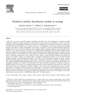
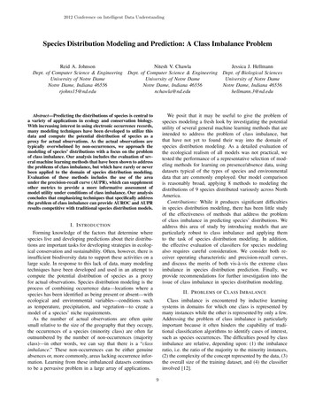
2012 Conference on Intelligent Data UnderstandingFigure 1. V. olivaceus distribution predicted by MAXENT (left) and HDDT (right).Figure 2. V. olivaceus distribution predicted by the other six evaluated models: C4.5 (top left), LR (top center), NB (topright), RF (bottom left), RF-SMT (bottom center), and CART (bottom right).and boasts the highest average AUPR by a large margin.The dominant performance of HDDT with respect to AUPRis particularly important, as AUPR may a useful metric for evaluating imbalanced species distribution models.In particular, the AUPR scores reflects negatively uponclassifiers that generate an imbalance between correctlypredicted occurrences—true positives—and incorrectly predicted occurrences—false positives. When dealing with imbalanced datasets, classifiers that are sensitive to this imbalance may capture true positives at the cost of a proportionally high number of false positives, resulting in a lowerAUPR score than a classifier that attempts to balance bothmeasures. In general, if we consider only the top-k classifierpredictions, we still find that MAXENT generates more falsepositive predictions than HDDT, resulting in a consistentlylower AUPR score.HDDT also performs well with respect to the CORRmetric. While both AUROC and AUPR performance onindividual datasets tended to be dominated by one or afew models, several different models dominate CORR ondifferent datasets. That said, HDDT produced the highestCORR on 4 of the 9 datasets, and also demonstrated thehighest average CORR.Though the success that HDDT demonstrates with boththe AUPR and CORR metrics suggests that the model iscapturing useful information regarding the minority class, itis important that the method produces distribution maps thatproperly model the species in question.14

2012 Conference on Intelligent Data UnderstandingThe distributions produced by MAXENT and HDDT arestrikingly different. HDDT is extremely conservative in itspredictions, generally giving high probabilities only to asmall region of the study area. This results in strong predictions only around individual occurrence localities. Thismay also explain its high AUPR performance, as by makingfewer predictions than MAXENT, HDDT is less likely toproduce false positive predictions, which are assigned agreater penalty by AUPR than by AUROC. In contrast,MAXENT is less particular, covering a large region of thestudy area with moderate probabilities.Although the difference in predicted area might stem frompredictions that are scaled in different ways, the variationin AUROC suggests actual differences between the methods. The conservative predictions allow HDDT to properlyexclude regions of the Great Lakes, which MAXENT includes in its prediction. Additionally, as MAXENT tendsto produce more false positive predictions than HDDT, itultimately receives a lower AUPR score. However, as thereis ambiguity as to which points represent true absence (andwhich represent assumed absence), we conjecture that AUPRmay underpredict the true classifier performance.the data, it is possible that a poorly fitted model (overestimating or underestimating all the predictions) has a gooddiscriminatory power. It is also possible that a well-fittedmodel has poor discrimination if, for example, probabilitiesfor presences are only moderately higher than those forabsences. In this way, it is possible for C4.5, which maynot properly model any imbalance or incompleteness in thedistribution, to nonetheless discriminate between presencesand absences relatively well. In contrast, MAXENT, whichattempts to model the occurrence localities as samples ina statistical distribution, may successfully model the imbalance and incompleteness of a species distribution whileproviding less discriminatory power. That is, it models thedistribution more accurately, but is less accurate at properlydistinguishing between points in that distribution.This provides evidence of a fundamental drawback ofAUROC in this domain: that it can present an overlyoptimistic view of an algorithm’s performance if there isa large skew in the class distribution. As species data arealmost universally imbalanced, due typically to a relativelylarge study area with a comparatively few presence localities and incomplete sampling, this limitation of the metricis invariably extenuated. To partly address this issue, wepropose the use of the AUPR metric to supplement theuse of AUROC. AUPR can better capture this imbalance,allowing it to provide a more informative picture of analgorithm’s performance under extreme imbalance. HDDTgenerally sees the highest boost in performance on datasetswith less imbalance.B. Broad PatternsBoth MAXENT and HDDT performed relatively wellaccording to all three evaluation measures. C4.5 and LRdemonstrated slightly lower performance, followed by RF,RF-SMT, and CART. NB showed intermediate performancefor AUROC, but the lowest AUPR and CORR performance.For most methods, predictive performance did not varyconsistently with number of presence records available formodeling.In general, we find that C4.5 tended to show the best AUROC performance on the datasets with the most occurrencesper area (and hence the least imbalanced). However, whenevaluated with respect to AUPR, C4.5 tended to performpoorly. Similarly, NB performed relatively well accordingto AUROC, yet was among the lowest performers withrespect to AUPR and CORR. In contrast, the models thatperformed well according to AUPR also tended to performwell according to AUROC and CORR.We find that, altogether, MAXENT and HDDT tend tooutperform the other methods, though C4.5 occasionallyboasts the highest AUROC. However, C4.5 tended to produce a high AUROC on datasets with low class imbalance,indicating that C4.5 is significantly skew-sensitive. Conversely, MAXENT demonstrated the highest AUROC fornearly all of the small, significantly imbalanced datasets.HDDT produced the most stable performance, when averaged over all of the datasets.As AUROC is a discrimination metric that represents thelikelihood that a presence will have a higher predicted valuethan an absence regardless of how well the predictions fitVI. C ONCLUSIONSWe can draw two major conclusions from our results.First, the precision-recall metric can be a useful tool forevaluating species distribution models. It is a skew-sensitivemetric that appears to have discriminatory power, and cancomplement the prevalent use of AUROC. Second, theHDDT model, which has been effective when used onimbalanced datasets in other domains, generally modeledspecies with performance competitive with MAXENT, anestablished species distribution model. Though HDDT originated in another discipline and has had little exposure inecological analysis, it appears to offer considerable promiseacross a much broader range of species data, providing anexciting avenue for future research.Class imbalance continues to be a significant problemfor species distribution modeling, as it pertains to boththe development and evaluation of these models. ThoughAUROC serves as

with SMOTE applied (RF-SMT) [3]. Each model can be considered to use some rules or mathematical algorithms to dene the ecological niche of the species based on the distribution of the species records in the environmental space. Once the predicted species niche is dened, the projection of the model into the geographical space produces a .