Transcription
Flow simulation with SolidWorksAkvile JonuskaiteBachelor ThesisFörnamn EfternamnPlastics Technology2017
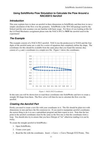
DEGREE THESISArcadaDegree Programme:Plastics TechnologyIdentification number:Author:Title:16576Akvile JonuskaiteFlow Simulation with SolidWorksSupervisor (Arcada):Mathew VihtonenCommissioned by:Arcada University of Applied SciencesAbstract:The idea of this thesis is to design a pipe system and run a flow simulation for the observation of the flow of fluids in pipes and compare it with the results obtained in the laboratory.First, a pipe system was modelled in SolidWorks software. Separate parts were designed,and then brought together into the final assembly.Secondly, an experimental analysis was performed in Heat Transfer laboratory. Volumetricflow rate was obtained using flow meter. This value was used in a velocity calculation.Finally, fluid flow simulations were performed using FloXpress and Flow Simulation addins. Different velocity and pressure magnitudes were observed along the pipeline.The average velocity in experimental analysis was found to be 0.531 m/s while the averagevelocity from Flow Simulation depending on the boundary conditions were 0.532 m/s and1.375 m/s respectively. Head loss was also calculated for experimental and Flow Simulation values. Head loss from laboratory experiment was calculated to be 2.446 m. Head losscalculated from Flow Simulation values depending on boundary conditions were 0.409 mand 2.428 m respectively.Keywords:SolidWorks, Turbulent flow, Laminar flow, Bernoulli’sequation, Velocity, Pressure, Head lossNumber of pages:Language:Date of acceptance:49English
CONTENTS12INTRODUCTION . 71.1Background . 71.2Objectives . 7LITERATURE REVIEW . 82.1Bernoulli’s Equation . 82.2Types of flow . 92.2.1Laminar flow . 102.2.2Turbulent flow . 102.2.3Transitional flow . 112.2.4Reynolds number . 112.3Entrance Region . 122.4Entry length . 132.5Head Loss in piping systems . 142.5.1Laminar flow . 152.5.2Turbulent flow . 152.5.3Major Head Loss . 152.5.4Minor Head Loss . 162.5.5Factors that affect head loss . 162.6Navier-Stokes equations . 172.7Friction factor . 182.7.1The laminar friction . 202.7.2The turbulent friction . 202.5.2.1The Colebrook equation . 202.5.2.2Moody chart . 202.83SolidWorks . 212.8.1Simulation add-ins . 212.8.2Standard parts . 22Method. 233.1The design of the pipe system . 233.1.1Weldments . 233.1.2Custom parts . 233.1.3The assembly of the pipe system . 263.2FloXpress Analysis . 27
3.2.1Simulation 1 . 283.2.2Simulation 2 . 283.33.3.1Simulation 1 . 303.3.2Simulation 2 . 323.44Flow Simulation . 28Laboratory experiment . 34RESULTS . 364.1Laboratory experiment calculation . 364.2FloXpress Analysis . 384.3Flow Simulation . 395DISCUSSION . 426CONCLUSION. 45References . 47
FiguresFigure 1 Laminar flow [5] . 10Figure 2 Turbulent flow [5] . 11Figure 3 The development of the velocity boundary layer in a pipe [6] . 13Figure 4 The variation of wall shear stress in the flow direction for flow in a pipe fromthe entrance region into the fully developed region [7] . 14Figure 5 Relative roughness for various pipes [15]. 19Figure 6 Moody Chart [14]. 21Figure 7 Pipe. 23Figure 8 On the left: opened valve. On the right: closed valve . 24Figure 9 Exploded view of the valve . 25Figure 10 Elbow . 26Figure 11 The complete pipe system . 26Figure 12 Lid. Extruded Base feature . 27Figure 13 Inlet and outlet boundary conditions . 28Figure 14 Mesh . 30Figure 15 Pressure contour . 31Figure 16 Velocity magnitude . 31Figure 17 Flow trajectories . 32Figure 18 Pressure contour . 33Figure 19 Velocity magnitude . 33Figure 20 Flow trajectories . 34Figure 21 Velocity magnitude . 39Figure 22 Cut plots. Velocity . 40Figure 23 Chart graph of average velocities obtained from Experimental and SolidWorkssimulation . 42
TablesTable 1 Values for calculation . 36Table 2 FloXpress simulation results . 39Table 3 Flow Simulation results . 41Table 4 Average velocities obtained from Experimental and SolidWorks simulation . 42Table 5 Head loss . 43Table 6 The velocities obtained from experimental and COMSOL simulation [26] . 43EquationsEquation 1: Conservation of energy . 8Equation 2: Work relating force and distance . 8Equation 3: Work relating pressure, area, and distance . 8Equation 4: Work relating pressure and volume . 8Equation 5: Work done . 8Equation 6: Kinetic energy . 8Equation 7: Potential energy. 8Equation 8: Bernoulli’s equation . 9Equation 9: Extended Bernoulli’s equation . 9Equation 10: Reynold’s number for circular pipes . 11Equation 11: Entry length. Laminar flow . 13Equation 12: Entry length. Turbulent flow . 13Equation 13: Total head loss . 14Equation 14: Head loss. Laminar flow . 15Equation 15: Head loss. Turbulent flow . 15Equation 16: Major head loss . 15Equation 17: Minor head loss . 16Equation 18: Continuity . 18Equation 19: Navier-Stokes . 18Equation 20: Reynold’s number for laminar flow . 20Equation 21: The Colebrook equation for transitional and turbulent flows . 20
List of symbolsNameSymbolUnit1.Acceleration due to olumetric flow rateV̇m3/s14.Dynamic viscosityμPa·s15.Kinematic viscosityvm2/s16.Head lossHLm17.Reynolds n factorf-22.Minor head loss coefficientk-
FOREWORDI would first like to thank you my thesis supervisor Mathew Vihtonen for advice andexcellent supervision throughout this thesis.I would also like to express my gratitude to all the professors and technical staff for guidance during my studies.Lastly, I would like to thank you my friends and family for their continuous support, andunlimited encouragement, particularly during the completion of this thesis.
1 INTRODUCTIONThe purpose of this study is to simulate flow in pipes utilizing SolidWorks software. Fluidflow may be very hard to predict and differential equations that are used in fluid mechanics are difficult to solve. SolidWorks add-ins enable you to simulate flow of liquids andgases and efficiently analyse the effects of fluid flow.1.1 BackgroundThe motion of a fluid is usually very complex. The observed fluid flow behaviour becomes much more understandable after defining the flow into laminar or turbulent regimes. The momentum equation provides one of the most recurring tools to be used inunderstanding fluid flows. Another fundamental tool for fluid flow analysis is continuityequation, both in its volumetric and its more widely applicable mass flow form.Along with the energy equation, the aforementioned equations, momentum and continuity, are also known as Navier – Stokes equations. Newtonian fluid flow is incompressiblewhen the density is constant. In such case Navier - Stokes equations can be simplified.1.2 ObjectivesThe objectives of this thesis are as follows:1. Model a pipe system using SolidWorks.2. Simulate and analyse the fluid flow in pipes using the SolidWorks Flow Simulation add-in and FloXpress.3. Compare experimental and simulated results obtained from SolidWorks andCOMSOL.7
2 LITERATURE REVIEW2.1 Bernoulli’s EquationThe application of the principle of conservation of energy leads to a relation betweenpressure, elevation and flow velocity in a fluid. This relation is called Bernoulli’s equation. [1] It is one of the best-known and widely-used equations in fluid mechanics.Bernoulli's equation can be viewed as a conservation of energy law for a flowing fluid.𝑊𝑜𝑟𝑘 𝑑𝑜𝑛𝑒 𝐾𝑖𝑛𝑒𝑡𝑖𝑐 𝐸𝑛𝑒𝑟𝑔𝑦 𝑃𝑜𝑡𝑒𝑛𝑡𝑖𝑎𝑙 𝐸𝑛𝑒𝑟𝑔𝑦 𝑊 (𝐾𝐸 𝑃𝐸)(1)Work done equals force multiplied by distance:𝑊 𝐹𝑑(2)We can plug in the formula that relates pressure and force, which gives us:𝑊 𝑝𝐴𝑑(3)Where A represents area.Volume is derived by multiplying area and height (distance), thus:𝑊 𝑝𝑉(4)Work done is equal to: 𝑊 𝑝1 𝑉1 𝑝2 𝑉2(5)Kinetic energy is the energy of mass in motion:𝐾𝐸 𝑚𝑣 22 𝜌𝑉𝑣 22(6)Where V represents volume.Potential energy is dependent on height:𝑃𝐸 𝑚𝑔𝑦 𝜌𝑉𝑔𝑦(7)Where y represents height.8
Substituting gives:ρVv22ρVv12p1 V p2 V ρVgy2 ρVgy122Divide by V:ρv22ρv12p1 p2 ρgy2 ρgy122Rearranging the formula to put the terms that refer to the same point on the same side ofthe equation:11𝑝1 2 𝜌𝑣12 𝜌𝑔𝑦1 𝑝2 2 𝜌𝑣22 𝜌𝑔𝑦2(8)Bernoulli’s equation has some restrictions: Steady flow Incompressible flow (which also means density is constant) Frictionless flow Flow along a streamline [2]In practical situations, problems may be analysed using extended Bernoulli’s equation:11𝑝1 2 𝜌𝑣12 𝜌𝑔𝑦1 𝑝2 2 𝜌𝑣22 𝜌𝑔𝑦2 𝐻𝐿(9)Where,HL – head losses due to friction or viscosity.y1 and y2 – heights of inlet and outlet2.2 Types of flowThere are three flow regimes. When a flow moves on in a tranquil fashion it is said to bestreamline or laminar flow, because the various axial layers in the fluid remain intact asthe flow proceeds. The so-called turbulent flow is chaotic, because layers in the flowconduit do not remain intact but are constantly being mixed due to turbulence, that is,9
chaotic motions in the flow. [3] Transitional flow is a mixture of laminar and turbulentflows.2.2.1 Laminar flowLaminar flow is characterized by smooth streamlines and highly ordered motion. If thepipe is sufficiently long (relative to the entry length) then the entrance effects are negligible and therefore the flow is fully developed. Laminar flow occurs when the fluid flowsin parallel layers without mixing. The velocity of the fluid is constant at any given moment. Since the flow is steady, there is no acceleration. The flow is laminar for cylindricalpipes when Reynolds number is less than 2300. [4]Figure 1 Laminar flow [5]2.2.2 Turbulent flowTurbulent flow is characterized by velocity fluctuations and highly disordered motion.Most flows encountered in practice are turbulent. Turbulent flow occurs when streamlinesof the liquid are irregular and change over time. The paths of the fluid flow are also irregular and form tiny whirlpool regions. [1] The flow is turbulent when Reynolds numberis greater than 4000. In practice, most flows in engineering are turbulent. However, thetheory of turbulent flow remains underdeveloped since this flow is a very complex mechanism dominated by fluctuations. Therefore, turbulent flow is analysed by applying experimental measures. [4]10
Figure 2 Turbulent flow [5]2.2.3 Transitional flowThe transition from laminar to turbulent flow is not sudden. It occurs over some region inwhich turbulent flow in the centre of the pipe and laminar flow is near the edges of thepipe. The flow fluctuates between laminar and turbulent flows before it becomes fullyturbulent. The flow is considered transitional when Reynolds number is in between 2300and 4000. [4]2.2.4 Reynolds numberReynolds number can reveal whether flow is laminar or turbulent. The transition fromlaminar to turbulent flow depends on the surface roughness, flow velocity, geometry, surface temperature, and type of fluid, among others. Flow regime mainly depends on theratio of inertial forces to viscous forces in the fluid. This ratio is called Reynolds numberand is expressed as𝑅𝑒𝐷 𝐼𝑛𝑒𝑟𝑡𝑖𝑎𝑙 �� 𝑓𝑜𝑟𝑐𝑒𝑠 𝑉𝑎𝑣𝑔 𝐷𝑣 𝜌𝑉𝑎𝑣𝑔 𝐷𝜇(10)Where,ReD Reynolds number for cylindrical pipe. Reynolds number is a dimensionless numberVavg average flow velocity (m/s)D diameter (m)v kinematic viscosity of the fluid (m2/s)µ dynamic viscosity (Pa·s)11
Critical Reynolds number Recr is the number at which the flow becomes turbulent. Thevalue of this number is different for different geometries and flow conditions. The generally accepted value of the critical Reynolds number for internal flow in a circular pipe isRecr 2300.Under most practical conditions, the flow in a circular pipe is: Laminar when Re 2300 Transitional when 2300 Re 4000 Turbulent when Re 4000 [4]2.3 Entrance RegionEntrance region is a region where the fluid enters a pipe at uniform velocity. The fluidparticles that are in contact with the surface of a pipe comes to a complete stop becauseof the no-slip condition. Because of friction, fluid particles in the adjacent layers gradually slow down. To make up for this velocity reduction, the velocity of the fluid at themidsection of the pipe increases to keep the mass flow rate through the pipe constant. Thearea of the flow in which the effects of the viscous shearing forces due to viscosity arefelt is known as the velocity boundary layer. The hypothetical boundary layers can bedivided into: The boundary layer region, where viscous effects and the velocity are considerable. Irrotational flow region, where frictional effects are negligible and velocity is constant in radial direction.The region of boundary layer increases in the flow direction until it merges with the layerfrom the opposite side at the centreline. The region starting from the pipe inlet to themeeting point of the two boundary layers is known as hydrodynamics entrance region andthe length of this region is called hydrodynamic entry length. Flow in the entrance regionis called hydrodynamically developing flow. The region at the merging point of boundarylayers is called hydrodynamically fully developed region. The flow is considered to befully developed until change in temperature in the fluid occurs. [4]12
Figure 3 The development of the velocity boundary layer in a pipe [6]2.4 Entry lengthThe length of hydrodynamics entrance region is called entry length. It may also be takenas the distance from the fluid entrance to 2% of the fully developed wall shear stressvalue. In laminar flow the hydrodynamic entry length is given as:𝐿ℎ 𝑙𝑎𝑚𝑖𝑛𝑎𝑟 0.05𝑅𝑒𝐷(11)In turbulent:𝐿ℎ 𝑡𝑢𝑟𝑏𝑢𝑙𝑒𝑛𝑡 10𝐷(12)13
Figure 4 The variation of wall shear stress in the flow direction for flow in a pipe from the entrance region into thefully developed region [7]2.5 Head Loss in piping systemsWhen fluid flows inside a pipe, friction occurs between the moving fluid and the stationary pipe wall. Some of the fluid’s hydraulic energy is converted to thermal energy due tothis friction. This process is irreversible therefore the fluid experiences a drop in pressure.This conversion and loss of energy is known as head loss. [8]Total head loss can be expressed as:𝐻𝐿 𝐻𝑚𝑎𝑗𝑜𝑟 𝑙𝑜𝑠𝑠𝑒𝑠 𝐻𝑚𝑖𝑛𝑜𝑟 𝑙𝑜𝑠𝑠𝑒𝑠14[9](13)
2.5.1 Laminar flowThe following equation is called Hagen-Poiseuille’s equation and is used for head losscalculation of steady laminar flow of incompressible fluid. 𝑝𝐻𝐿 𝜌𝑔(14)Where,HL head loss (m)p pressure (Pa)ρ density (kg/m3)g acceleration due to gravity (g 9.81 m/s2) [4]2.5.2 Turbulent flowIn turbulent flow, whirlpools and wakes make the flow unpredictable. The formula belowis called Darcy’s equation and is used for the calculation in fully developed flow:2𝐿 𝑉𝑎𝑣𝑔𝐻𝐿 𝑓 𝐷(15)2𝑔Where,f friction factor related to the roughness inside the pipeL length of the pipe (m)D internal diameter of the pipe (m)Vavg average liquid velocity (m/s)g acceleration due to gravity (g 9.81 m/s2) [4]2.5.3 Major Head LossMajor losses are associated with energy loss per length of pipe. It is caused by friction inpipes and ducts.2𝐿 𝑉𝑎𝑣𝑔𝐻𝐿 𝑚𝑎𝑗𝑜𝑟 𝑓 𝐷2𝑔(16)15
Where,f friction factorL pipe length (m)Vavg average velocity (m/s)D internal diameter (m)g acceleration due to gravity (g 9.81 m/s2) [10]2.5.4 Minor Head LossMinor losses are associated with technological equipment. It is caused by componentssuch as valves, bends, tees, etc. Minor losses can easily exceed major losses in relativelyshort pipe systems with a relatively large amount of bends and fittings. [10]𝐻𝐿 𝑚𝑖𝑛𝑜𝑟 𝑘2𝑉𝑎𝑣𝑔2𝑔(17)Where,k minor head loss coefficient [11]2.5.5 Factors that affect head loss1. Flow Rate.The velocity of the liquid increases at the same rate as the flow rate. Due to viscosity,the resistance to flow also increases. The head loss is proportional to the square of thevelocity therefore the increase in loss is very rapid.2. Inside diameter of the pipe.The velocity of the liquid is reduced when the flow area increases, which happenswhen the inside diameter is larger. Head loss due to friction is reduced when velocitydecreases. However, the flow area decreases if the inside diameter of the pipe is reduced, in such case the velocity of the liquid increases and the head loss due to frictionincreases.16
3. Roughness of the pipe wall.The roughness of the inside pipe wall increases with the thickness of non-movingboundary layer increase. The resulting reduction in flow area causes the rise of thevelocity of the liquid which in turn increases the head loss due to friction.4. Corrosion and Scale Deposits.Scale deposits and corrosion both increase the roughness of the inside pipe wall andthus increases head loss.5. Viscosity of the liquid.More energy is needed to move high viscosity liquid. The higher the viscosity of theliquid is, the more friction occurs.6. Length of the pipe.Head loss due to friction occurs all along a pipe. Therefore, head loss would be constant along the pipe at a given flow rate.7. Fittings.Fittings disrupt the smooth flow of the liquid. When the disruption occurs, head lossdue to friction occurs. However, elbows, tees, valves, and other fittings are necessaryto a piping system.8. Straightness of the pipe.Due to momentum, liquid travels in a straight line. Curved or crooked pipe disturbsstraight flow and thus increases the head loss due to friction. [12]2.6 Navier-Stokes equationsNavier-Stokes equations are the basis for nearly all CFD (Computational Fluid Dynamics) flow modelling. Solving these equations predicts the fluid velocity and its pressurein a given geometry. The Navier-Stokes equations are always solved together with thecontinuity equation. The Navier-Stokes equations serves as the conservation of momen17
tum, while the continuity equation represents the conservation of mass. [13] These equations apply to any point in the flow and thus all details of the flow can be solved everywhere in the flow domain. However, most differential equations in fluid mechanics arevery difficult to solve and therefore often require help from a computer. These equationsin certain cases may need to be combined with additional equations, such as energy equation. [4]Continuity equation: 𝜌 𝑡 (𝜌𝑣) 0(18)Navier-Stokes:𝛿𝑣𝜌 𝛿𝑡 𝑝 𝜌𝑔 𝜇 2 𝑣(19)Where,ρ fluid densityv fluid flow velocityp fluid pressureµ fluid dynamic viscosity del operator [4]2.7 Friction factorThe friction factor is a dimensionless factor that depends primarily on the fluid velocity,pipe diameter, fluid density, and viscosity. It can also be a function of wall roughnesswhich depends on the size e. Thus, the general formula can be written as:𝑒𝑓 𝑅𝑒,𝐷Where e/D relative roughness, which is the ratio of the mean height of roughness of thepipe to the pipe diameter. [14]18
Figure 5 Relative roughness for various pipes [15]19
2.7.1 The laminar frictionThe laminar friction factor is a function of Reynolds number alone and is independent ofany other factor.64𝑓 𝑅𝑒[3](20)2.7.2 The turbulent frictionThe turbulent friction factor is influenced by both Reynolds factor and wall roughness.To determine friction factor, Colebrook equation and Moody chart are used.2.5.2.1The Colebrook equationIn 1939, Cyril F. Colebrook combined the available data for transition and turbulent flowin smooth and rough pipes into the following formula known as the Colebrook equation:1 𝑓 2 𝑙𝑜𝑔10 (2.5.2.2𝑒/𝐷3.7 2.51𝑅𝑒 𝑓)[4](21)Moody chartMoody chart is one of the most accepted and used charts in engineering. It relates theDarcy friction factor, Reynolds number and relative roughness. Moody friction factor canbe used in Darcy-Weisbach major loss equation. [4]20
Figure 6 Moody Chart [14]2.8 SolidWorksSolidWorks is a computer-aided design (CAD) software, which is used to create 2D or3D models. This simple and yet very powerful computer program enables designers tocreate highly detailed parts and assemblies as well as production-level drawings. SolidWorks is an excellent tool to cover a lot of stages of product development. Not only thissoftware provides with tools needed to generate complex surfaces, structural welded assemblies, and others, it also allows you to test your design before manufacture using broadrange of tools: fluid dynamics, static and dynamic response, heat transfer to name a few.[16]2.8.1 Simulation add-insSolidWorks has tools that enable you to simulate liquid and gas flow in real world conditions, run “what if” scenarios, and efficiently analyse the effects of fluid flow, heat transfer, and related forces on immersed or surrounding components. [17]FloXpress is a basic fluid flow analysis tool. It calculates how water or air flows throughpart or assembly models. It comes with all SolidWorks 3D CAD software packages. [18]21
More advanced, SolidWorks Flow simulation uses CFD (computational fluid dynamics)analysis, which simulates fluid passing through or around an object. The analysis maycontain unsteady and compressible flows, heat transfer, etc. in one calculation only. Suchcomplicated analysis may be very costly and time consuming without some form of simulation tool. [19]2.8.2 Standard partsSolidWorks provides with library toolbox of standard parts which helps the user to speedup the design process, increase productivity, and save both time and development costs.The components can be customized to meet your needs or can be used “as is”. Items canbe easily dragged and dropped into the assembly for further design processes. SolidWorkstoolbox includes machine compone
The purpose of this study is to simulate flow in pipes utilizing SolidWorks software. Fluid flow may be very hard to predict and differential equations that are used in fluid mechan-ics are difficult to solve. SolidWorks add-ins enable you to simulate flow of liquids and gases and efficiently analyse the effects of fluid flow. 1.1 Background