Transcription
Advanced RegressionwithJMP PROGerman JMP User MeetingHolzminden – June 22, 2017Silvio Miccio
Overview Introduction Some Details on Parameter Estimation and Model Selection Generalized Linear Models Penalized Regression Models in JMP PRO Example: Analysis of Time to Event Data (Parametric Survival Models) Classification Model with Missing Informative Data Linear Mixed Models in JMP PRO Example: Nested Intercept Repeated Measure (Consumer Research)
Introduction Multiple Linear Regression (MLR) is one of the mostcommonly used methods in Empirical Modeling MLR is high efficient as long as all assumptions are met Especially observational data often do not meet theassumptions, resulting in problems with estimation ofcoefficients and model selection and with this in modelvalidity Hence, Advanced Regression Methods, like available in JMPPRO, have to applied to benefit from the ease ofinterpretation of regression methods
Linear Regression yi xji β0 βj εi Response; i 1, 2 .n (n number of observations) Factor, Predictor; j 1, 2 .p (p number of factors) Intercept Coefficients Error
Assumptions1. Errors are normally distributed (0, )2. Errors are independentE.g. no pattern in residuals over time or groups3. HomoscedasticityVariance is constant in the entire model space4. Factors are not or only slightly correlatedRule of thumb VIF 3 or 55. Predictors are fixed factors, measured with almost “no” error.Error is assumed to be completely on the side of the residuals6. Response is a linear combination of coefficients and factors
Some Details on LinearRegressionParameter Estimation
Linear RegressionFor generalization of the parametric model of a linear regression it makes sense to change to matrix notation:y Xβ εn 1 vector of responses1 1. . . . ." . . . . . . . . .1 ! ! ! p 1 vector ofunknown constants& & !with ! n p matrix of thefactors/variablesn 1 vector of random errors N (0,σ2)
Standard Least Square Estimate!: ? L &’&L (y - Xβ)‘(y - Xβ)L y’y - β‘X‘y - y‘X β β‘X‘X βL y’y - 2β‘X‘y β‘X‘X β9: 2X y 2X Xβ9X’X β X‘yβ (X‘X)-1X‘y(AB)‘ B‘A‘β‘X‘y y‘X βQuadratic Function9: 09
X Matrix (coded) – 23 FF Design 3 Center PointsInt X1 X2 X3 X1X2 X1X3 X2X31 -1 -1 -111 -1 -1111-1-111 -11 -1-11-111 -11-1-111 -1 -111-1-111-11-1X 1 -11 -111-1-111111111100000010000001000000 X matrix of a full factorial23 design with threecenter points 1st column intercept 2nd – 4th column maineffects 5th – 7th columninteractions
X’X (Covariance Matrix)
(X’X)-1 Inverted Covariance 00000001/800000001/8 The “degrees of freedom“ for estimating the model coefficients show up at thediagonal This is only true if all off diagonal elements are 0 (all factors are independent ofeach other) When off diagonal elements are not zero then the factors are correlated
MulticollinearityOrthogonal
Effects of Multi-Co-linearity Singular matrix no solution High variance in the coefficients High variance in the predictions Often high R-square, but (all) factors are insignificant Small changes in the data may have a big effect on thecoefficients (not robust) Best subset selection i.e. via Stepwise Regression maybecome almost impossible
Some Details on LinearRegressionModel Selection
Model Selection Overall goal in Empirical Modeling is to identify the model withthe lowest expected prediction errorExpected Prediction Error Irreducible error (inherent noise of the system)Squared Bias (depends on model selection)Variance (depends on model selection) This requires to find the model with optimum complexity (e.g.number of factors, number of sub-models, functional form ofmodel terms, modeling method) Model Selection: “estimating the performance of differentmodels in order to choose the (approximate) best one”
Bias-Variance Trade Off Training error: variation in the datanot explained by the model Test error: expected prediction errorbased on independent test data If model complexity is too lowthe model is biased (importantfeatures of the system notcaptured by the model) If model complexity is too highthe model is fit too hard to thedata, which results in a poorgeneralization of the prediction(high prediction variance) The challenge is to identify themodel with the optimum tradeoff between bias and variance
Methods for Model Selection When it is not possible to split the data into a training,validation and test set (this is the case for designedexperiments or for small data sets) model selectioncan be done by via measures that try to approximatingthe validation/test error, like AIC, AICc and BIC Here the estimated value usually is not of directinterest, it is the relative size that matters Alternative methods based on re-sampling (e.g. crossvalidation) provide direct estimate of the expectedprediction error (can be used for model assessment)
Generalized Linear ModelsModeling discrete responses and non-normal distributederrors
Generalized Linear Model (GLM) A GLM is a generalization of a linear model for non-normalresponses where errors being a function of the meano Binomial - dichotomous data (yes/no, pass/fail)o Poisson - count datao Log Normal - data restricted to non-negative values (transformed datanormally distributed)o and much more Components of GLM1. Random Component2. Systematic Component3. Link Function
Random ComponentIdentifies the distribution and variance of the response.Usually derives from the exponential family of distributions,but not restricted to it.The parameter θi and φ are location and scale parameter
Systematic Component & Link FunctionSystematic ComponentLinear function of the factors, the so called Linear Predictorwhere the predictors can be transformed (squared, log )A Link FunctionSpecifies the link between random and systematiccomponents. It is an invertible function that defines therelation between the response and the linear predictorA B BC A
Common Variance and Link Functions
Comparison Standard Least Squares vs. GLMStandard Least Square Regression " & " " C " Iteratively Re-Weighted Least Squares BC AA " & " E" C " Ezy is an n 1 vector of responsesX is an n p matrix of the factors variablesβ is a p 1 vector of unknown constantsε is an n 1 vector of random errors N (0,σ2)X′ is the transpose of XX X′ is a p p matrix of correlations between the factorsη is the linear predictorg-1 is the inverse link functionW is a diagonal matrix of weights wiz is a response vector with entries zi
Generalized Linear RegressionPenalized Regression
Generalized Linear Regression (GLR)GLR can be seen as extension of GLM, in addition being ableto deal with: Multicollienearity and to perform Model Selection (p n/2 as well as for p n)This is achieved by penalized regression methods, whichattempt to fit better models by shrinking the parameterestimatesAlthough shrunken estimates are biased, the resultingmodels are usually better i.e. having a lower prediction error
Ridge Regression Ridge Regression was developed as remedy for multicollinearity It attempts to minimize the penalized residual sum of squaresG HIJ! KLBMN ? OO? O P O? O λ 0 is the regularization parameter controlling the amount ofshrinkage P O? Ois called the L2 penalty, due to the squared term
Ridge Regression Parameters are estimated according to:G HIJ S S TUC S Vwhere I is a p x p diagonal identity matrix (diagonalelements are 1 and all off diagonal elements are 0 When there is a multicollinearity problem the off diagonalelements (covariances) of (X’X) are large compared to thevalues of the diagonal (variances) By adding λI to the covariance matrix, the diagonal elementsincrease
What is Ridge Regression Doing? Since β (X’X λI)X’X λI)-1X’y,X’y the diagonal elements of the invertedmatrix are getting smaller, which means the parameterestimates for β are shrunken As λ gets larger the inverse is getting smaller meaning thevariance in β decreases (what is desired), but only to a certainpoint When λ is getting too big the residual sum of squares increase,because the coefficients are shrunken so much that they do notexplain the response anymore (bias) Hence there is an optimum for λ
LASSO Regression Since Ridge Regression is shrinking large coefficients, which arepotentially important, more than small coefficients the LASSO wasdeveloped LASSO shrinks all coefficients by the same amount, but in additionshrinks “unimportant” factors to exactly zero, which means they areremoved from the model ( Model SelecQon) Like Ridge Regression, LASSO minimizes the error sum of squares, butusing a different penaltyWXYYZ! KLBMN ? OO? O P O? O
LASSO Regression P O? O is called the L1 penalty, due to the “first power” inthe penalty term Parameter estimation for the LASSO is algorithmic, becausethere is no closed from solution (penalty is an absolute value,cannot be differentiated) The Lasso is designed for model selection, but is not doing thatgood with collinearity Ridge is designed for multicollinearity, but is doing no modelselection Hence, a combination of both methods would be desired
Elastic Nets[\! KLBMN ? OO? O P O? O P O? O Elastic Nets combine the L1 and the L2 penalty The L1 penalty controls the model selection The L2 penaltyo Enables p no Keeps groups of highly correlated variables in the model (LASSO just picks onevariable from the group)o Improves, smoothes parameter estimation
Adaptive Methods Adaptive methods penalize “important” factors less than“unimportant” by a weighted penalty Adaptive L Penalty P OO? O O Adaptive L Penalty P O? O Ois the maximum likelihood estimate if existing, for normaldistributed data the least square estimate or for non normaldistributed data the ridge solution Adaptive models attempt to ensure Oracle Properties Identification of true active factors Correct estimation of parameter estimates
Tuning Parameters (from JMP Help) LASSO and Ridge are determined by one tuning parameter (L1 or L2) Elastic Nets are determined by two tuning parameters (L1 and L2),where the Elastic Net Alpha is the weight between the penalties The higher the tuning parameter, the higher the penalty (adding azero provides the Maximum Likelihood solution (MLE); no penalty)o When tuning parameter is too small the model is likely to overfito When tuning parameter is too big there is bias in the model To obtain a solution the tuning parameter is increased over a fine grid Optimum solution is where best fit over the entire tuning parametergrid is achieved
Tuning Parameters – Elastic Net Alphafrom JMP Help) Determines the mixbetween the L1 and L2penalty Default value is 0.9meaning (coefficient on L1penalty is set to 0.9,coefficient on L2 penalty isto 0.1 If Elastic Net Alpha is notset, the algorithmcomputes the Lasso, ElasticNet, and Ridge fits, in thatorder and keeps the “best”solution
Model Tuning Try different Estimation Methods,settings for Advanced Controls andValidation Methods to find best model All models are displayed in the modelreport and can be individually saved asscript and prediction formula Note: k-fold or random holdbackvalidation is not recommended forDOE data
Data Set 1 - Parametric Survival Analysis 4 Factors (E Equipment Set-Up, P Process Setting, F1 & F2 ProductFormulation) have been investigated in a designed experiment Column Censor includes the censoring variable (0 no censoring, 1 censoring) Response is the time the sample resists a force applied to it For feasibility reasons the measurement is stopped after a pre-definedmaximum test time. This leads to so called “right censoring”, because notall samples fail within the maximum test time. Objective is to create a model for predicting the survival time of thesample The data file “GLR Survival” contains the scripts for the parametricsurvival model for JMP (does not allow for automated model selection)and JMP PRO
Data 2 - Credit Risk Scoring The data set is called Equity.jmp and taken from the JMP Sample Data Library located in the JMP Helpmenu It is based on historical data gathered to determine whether a customer is a good or bad credit risk for ahome equity loan (watch out: missing data, they are set to Informative Missing in JMP PRO, becausethey contain important information) Predictors: NODEBTINC how much was the loan how much they need to pay on their mortgage assessed valuation reason for loan broad job category years on the job number of derogatory reports number of delinquent trade lines age of oldest trade line number of recent credit enquiries number to trade lines dept to income ratio Response is Credit Risk, predict good and bad credit risks Data file “Credit Risk” contains scripts for JMP PRO (GLR for model selection, informative missing,validation column) and JMP (logistic regression, it is possible to do stepwise and manual informativemissing coding – see JMP home page for details)
Linear Mixed ModelsG-Side and R-Side Random Effects
Fixed Factors Usually the factors e.g. in a design of experimentare varied within fixed factor levels With fixed factors we can make statistical inferenceswithin the investigated model space, based on thefactor effects When the factor levels are randomly chosen from alarger population of factor levels, the factor is saidto be a random factor
Random Factors Random factors allow to draw conclusions about the entirepopulation of possible factor levels The population of possible factor levels is considered to beinfinite Random effects models are of special interest for identifyingsources of variation, because they allow to identify variancecomponents Random Factors Random Effects: Machines, Operators, Panelists Random Effects also have to be considered for split plot designs,correlated responses, spatial data, repeated measurements
Random Effects Model " bc &c 0, d , & 0, ef " ; h bdb e y is an vector of responses X is the regression matrix of the fixed effects β is a vector of unknown fixed effectparameters Z is the regression matrix of the of therandom effects γ is a vector of unknown random effectsparameters ε is a vector of random errors (not requiredto be independent or homogenous) G is variance-covariance matrix for randomeffects R is variance-covariance matrix for modelerrors G-side effects are specified by the Z matrix(random effects) R-side effects, are specified by thecovariance structure (repeated structure)
Repeated Covariance Structure Requirements(taken from JMP Help)For details regardingdifferent covariancestructures, please seethe JMP Help
Strategies for Selecting Covariance Structure It is “always” possible to fit an unstructured covariancestructure, but this also means fitting the most complexmodel (potential risk of overfitting) Best option is to use covariance structure that are expectedto make sense for the given context (see JMP for detailsregarding the structures) To find out the best covariance structure from competingmodels AICc and/or BIC can be used Check the structure of the residuals by plotting them orusing the variogram
Repeated Measures (from JMP Help) Repeated measures designs, also known as within-subject designs,model changes in a response over time or space while allowing errors tobe correlated. Spatial data are measurements made in two or more dimensions,typically latitude and longitude. Spatial measurements are oftencorrelated as a function of their spatial proximity. Correlated response data result from making several measurements onthe same experimental unit. For example, height, weight, and bloodpressure readings taken on individuals in a medical study, or hardness,strength, and elasticity measured on a manufactured item, are likely tobe correlated. Although these measurements can be studied individually,treating them as correlated responses can lead to useful insights.
Correlated Response (Example from JMP Help)In this example, the effect of two layouts dealing with wafer productionis studied for a characteristic of interest. Each of 50 wafers ispartitioned into four quadrants and the characteristic is measured oneach of these quadrants. Data of this type are usually presented in aformat where each row contains all of the repeated measurements forone of the units of interest. Data of this type are often analyzed usingseparate models for each response. However, when repeatedmeasurements are taken on a single unit, it is likely that there is withinunit correlation. Failure to account for this correlation can result inpoor decisions and predictions. You can use the Mixed Modelpersonality to account for and model the possible correlation.P&G example cannot be shared. Use JMP data file “Wafer Stacked”from the JMP sample data library (not attached). Can be analyzed inJMP PRO only; R-Side Random Effect with spatial structure.
Advanced Regression with JMP PRO German JMP User Meeting Holzminden-June 22, 2017 Silvio Miccio. Overview Introduction Some Details on Parameter Estimation and Model Selection Generalized Linear Models Penalized Regression Models in JMP PRO Example: