WIXLIB

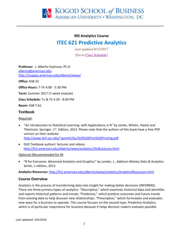
Chapter 5: Logistic Regression 9In the above paragraphs we spoke only of “odds”. Now let us calculate an “odds ratio”. Itis important to note that this can be done in two equivalent ways. Suppose we want toknow the odds ratio of passing the class by comparing those who pass the midterm(PassMidterm 1 in the numerator) to those who fail the midterm (PassMidterm 0 in thedenominator). The usual calculation leads to:Odds of passing the class; given passed the Midterm10 Odds of passing the class; given failed the Midterm3 50 8.33.265which has the following interpretation: the odds of passing the class are 8.33 times theodds of failing the course if you pass the midterm. This odds ratio can be converted into aprobability. We know that P(Y 1)/P(Y 0) 8.33, and by definition P(Y 1) P(Y 0) 1, sosolving two equations in two unknowns yields P(Y 0) (1/(1 8.33)) (1/9.33) 0.1072and P(Y 1) 0.8928. As a quick check, observe that 0.8928/0.1072 8.33. Note that thelog-odds is ln(8.33) 2.120. Of course, the user doesn’t have to perform all thesecalculations by hand; JMP will do them automatically. When a logistic regression hasbeen run, simply clicking on the red triangle and selecting “Odds Ratios” will do thetrick.Equivalently, we could compare those who fail the midterm (PassMidterm 0 in thenumerator) to those who pass the midterm (PassMidterm 1 in the denominator) andcalculate:Odds of passing the class; given failed the MidtermOdds of passing the class; given passed the Midterm2 5 6 1 0.12.10508.333which tells us that the odds of failing the class are 0.12 times the odds of passing the classfor a student who passes the midterm. Since P(Y 0) 1 - π (the probability of failingthe midterm) is in the numerator of this odds ratio, we must interpret it in terms of theevent failing the midterm. It is easier to interpret the odds ratio when it is less than 1 byusing the following transformation: (OR – 1)*100%. Compared to a person who passesthe midterm, a person who fails the midterm is 12% as likely to pass the class, orequivalently, a person who fails the midterm is 88% less likely, (OR – 1)*100% (0.12 –1)*100% -88%, to pass the class than someone who passed the midterm. Note that thelog-odds is ln(0.12) -2.12.The relationships between probabilities, odds (ratios), and log-odds (ratios) arestraightforward. An event with a small probability has small odds, and also has small logodds. An event with a large probability has large odds and also large log-odds.Probabilities are always between zero and unity; odds are bounded below by zero but canbe arbitrarily large; log-odds can be positive or negative and are not bounded, as shownKlimberg, Ron and B.D. McCullough. Fundamentals of Predictive Analytics with JMP.Copyright 2012, SAS Institute Inc., Cary, North Carolina, USA. ALL RIGHTS RESERVED.

Chapter 5: Logistic Regression 10in Figure 5.6. In particular, if the odds ratio is 1 (so the probability of either event is0.50), then the log-odds equals zero. Suppose π 0.55 so the odds ratio 0.55/0.45 1.222. Then we say that the event in the numerator is (1.222-1) 22.2% more likely tooccur than the event in the denominator.Different software packages adopt different conventions for handling the expression ofodds ratios in logistic regression. By default JMP has uses the “log odds of 0/1”convention which puts the “0” in the numerator and the “1” in the denominator. This is aconsequence of the sort order of the columns, which we will address shortly.To see the practical importance of this, rather than compute a table and perform the abovecalculations, we can simply run a logistic regression. It is important to make sure thatPassClass is nominal and that PassMidterm is continuous. If PassMidterm is nominal,JMP will fit a different but mathematically equivalent model that will give different (butmathematically equivalent) results. The scope of the reason for this is beyond this book,but interested readers can consult Help Books Modeling and Multivariate Methodsand refer to Appendix A.If you have been following along with the book, both variables ought to be classified asnominal, so PassMidterm needs to be changed to continuous. Right-click on the columnPassMidterm in the data grid and select Column Info . Beside Modeling Type, click onthe black triangle and select Nominal, then OK.Now that the dependent and independent variables are correctly classified as Nominaland Continuous, respectively, let’s run the logistic regression:Click from the top menu Analyze Fit Model. Click on PassClass and click on Y. ClickPassMidterm and click on Add. The Fit Model dialog box should now look like Figure5.7. Click Run.Klimberg, Ron and B.D. McCullough. Fundamentals of Predictive Analytics with JMP.Copyright 2012, SAS Institute Inc., Cary, North Carolina, USA. ALL RIGHTS RESERVED.

Chapter 5: Logistic Regression 11Figure 5.8 displays the logistic regression results.Klimberg, Ron and B.D. McCullough. Fundamentals of Predictive Analytics with JMP.Copyright 2012, SAS Institute Inc., Cary, North Carolina, USA. ALL RIGHTS RESERVED.

Chapter 5: Logistic Regression 12Klimberg, Ron and B.D. McCullough. Fundamentals of Predictive Analytics with JMP.Copyright 2012, SAS Institute Inc., Cary, North Carolina, USA. ALL RIGHTS RESERVED.

Chapter 5: Logistic Regression 13Examine the parameter estimates in Figure 5.8. The intercept is 0.91629073 and the slopeis -2.1202635. The slope gives the expected change in the logit for a one unit change inthe independent variable, i.e., the expected change on the log of the odds ratio. However,if we simply exponentiate the slope, i.e., compute e 2.1202635 0.12 , then we get the 0/1odds ratio.There is no need for us to exponentiate the coefficient manually. JMP will do this for us:Click on the red triangle and select Odds Ratios. The Odds Ratios tables are added to theJMP output as shown in Figure 5.9.Unit Odds Ratios refers to the expected change in the odds ratio for a one-unit change inthe independent variable. Range Odds Ratios refers to the expected change in the oddsratio when the independent variable changes from its minimum to its maximum. Sincethe present independent variable is a binary 0-1 variable, these two definitions are thesame. We get not only the odds ratio, but a confidence interval, too. Notice the rightskewed confidence interval; this typical of confidence intervals for odds ratios.To change from the default “log odds of 0/1” convention which puts the “0” in thenumerator and the “1” in the denominator, in the data table rightclick on the name of thePassClass colum. Under “Column Properties” select “Value Ordering”. Click on thevalue “1” and click “Move Up” as in Figure 5.10.Klimberg, Ron and B.D. McCullough. Fundamentals of Predictive Analytics with JMP.Copyright 2012, SAS Institute Inc., Cary, North Carolina, USA. ALL RIGHTS RESERVED.

Chapter 5: Logistic Regression 14Then, when you re-run the logistic regression, while the parameter estimates will notchange, the odds ratios will change to reflect the fact that the “1” is now in the numeratorand the “0” is in the denominator.The independent variable is not limited to being only a nominal (or ordinal) dependentvariable, it can be continuous. In particular, let’s examine the results using the actualscore on the midterm, MidtermScore as an independent variable:Click Analyze Fit Model. Click PassClass and click on Y and then click MidtermScoreand click on Add. Click Run.Klimberg, Ron and B.D. McCullough. Fundamentals of Predictive Analytics with JMP.Copyright 2012, SAS Institute Inc., Cary, North Carolina, USA. ALL RIGHTS RESERVED.

Chapter 5: Logistic Regression 15This time the intercept is 25.6018754 and the slope is -0.3637609, so we expect the logodds to decrease by 0.3637609 for every additional point scored on the midterm, asshown in Figure 5.11.To view the effect on the odds ratio itself, as before click on the red triangle and clickOdds Ratios. Figure 5.12 displays the Odds Ratios tables.MidtermScoreFor a one unit increase in the midterm score, the new odds ratio will be 69.51% of the oldodds ratio or, equivalently, we expect to see a 30.5% reduction in the odds ratio(0.695057 – 1)*100% -30.5%). For example, suppose a hypothetical student has amidterm score of 75%. His log odds of failing the class would be 25.6018754 –0.3637609*75 -1.680192, so his odds of failing the class would be exp(-1.680192) Klimberg, Ron and B.D. McCullough. Fundamentals of Predictive Analytics with JMP.Copyright 2012, SAS Institute Inc., Cary, North Carolina, USA. ALL RIGHTS RESERVED.

Chapter 5: Logistic Regression 160.1863382; that is, he is much more likely to pass than fail. Converting odds toprobabilities (0.1863328/(1 0.1863328) 0.157066212786159), we see that hisprobability of failing the class is 0.15707, and his probability of passing the class is0.84293. Now, if he increased his score by one point to 76, then his log odds of failingthe class would be 25.6018754 – 0.3637609*76 -2.043953. Thus, his odds of failing theclass becomes exp(-2.043953) 0.1295157. So, his probability of passing the class wouldrise to 0.885334, and his probability of failing the class would fall to 0.114666. Withrespect to the Unit Odds Ratio, which equals 0.695057, we see that a one unit increase inthe test score changes the odds ratio from 0.1863382 to 0.1295157. In accordance withthe estimated coefficient for the logistic regression, the new odds ratio is 69.5% of the oldodds ratio because 0.1295157/0.1863382 0.695057.Finally, we can use the logistic regression to compute probabilities for each observation.As noted, the logistic regression will produce an estimated logit for each observation.These can be used, in the obvious way, to compute probabilities for each observation.Consider a student whose midterm score is 70. His estimated logit is 25.6018754 –0.3637609(70) 0.1386124. Since exp(0.1386129) 1.148679 /(1- ), we can solvefor (the probability of failing) 0.534597.We can obtain the estimated logits and probabilities by clicking the red triangle on“Normal Logistic Fit” and selecting Save Probability Formula. Four columns will beadded to the worksheet: Lin[0], Prob[0] and Prob[1]. These give for each observation theestimated logit, the probability of failing the class, and the probability of passing theclass, respectively. Observe that the sixth student has a midterm score of 70. Look up hisestimated probability of failing (Prob[0]); it is very close to what we just calculatedabove. See Figure 5.13. The difference being the computer carries 16 digits through itscalculations, while we carried only six.Klimberg, Ron and B.D. McCullough. Fundamentals of Predictive Analytics with JMP.Copyright 2012, SAS Institute Inc., Cary, North Carolina, USA. ALL RIGHTS RESERVED.

Chapter 5: Logistic Regression 17The fourth column (Most Likely PassClass) classifies the observation either 1 or 0depending upon whether the probability is greater than or less than 50%. We can observehow well our model classifies all the observations (using this cut off point of 50%) byproducing a confusion matrix: Click on the red triangle and select Confusion matrix.Figure 5.14 displays the confusion matrix for our example. The rows of the confusion arethe actual classification, that is, whether PassClass is 0 or 1. The columns are thepredicted classification from the model, that is, the predicted 0/1 values from that lastfourth column using our logistic model and a cut point of .50. Correct classifications arealong the main diagonal from upper left to lower right. We see the model classified 6students as not passing the class, and actually they did not pass the class. The model alsoclassifies 10 students as passing the class when they actually did. The values on the otherdiagonal, both equal to 2, are misclassifications. The results of the confusion matrix willbe examined in more detail when we discuss model comparison in Chapter 9.Klimberg, Ron and B.D. McCullough. Fundamentals of Predictive Analytics with JMP.Copyright 2012, SAS Institute Inc., Cary, North Carolina, USA. ALL RIGHTS RESERVED.

Chapter 5: Logistic Regression 18Of course, before we can use the model we have to check the model’s assumptions, etc.The first step is to verify the linearity of the logit; this can be done by plotting theestimated logit against PassClass: Click on Graph Scatterplot Matrix. Click on Lin[0]and click Y, columns and click MidtermScore and click X. Click OK. As shown in Figure5.15, the linearity assumption appears to be perfectly satisfied.The analog to the ANOVA F Test for linear regression is found under the Whole ModelTest, shown in Figure 5.16, in which the Full and Reduced models are compared. Thenull hypothesis for this test is that all the slope parameters are equal to zero. SinceProb ChiSq is 0.0004, this null hypothesis is soundly rejected. For a discussion of otherstatistics found here, such as BIC and Entropy RSquare, see the JMP Help.Klimberg, Ron and B.D. McCullough. Fundamentals of Predictive Analytics with JMP.Copyright 2012, SAS Institute Inc., Cary, North Carolina, USA. ALL RIGHTS RESERVED.

Chapter 5: Logistic Regression 19The next important part of model checking is the Lack of Fit test. See Figure 5.17. Itcompares the model actually fitted to the saturated model. The saturated model is a modelgenerated by JMP that contains as many parameters as there are observations, and so fitsthe data very well. The null hypothesis for this test is that there is no difference betweenthe estimated model and the saturated model. If this hypothesis is rejected, then morevariables (such as cross-product or squared terms) need to be added to the model. In thepresent case, as can be seen, Prob ChiSq 0.7032. We can therefore conclude that we donot need to add more terms to the model.Let’s turn now to a more realistic dataset with several independent variables. During thisdiscussion we will also present briefly some of the issues that should be addressed andsome of the thought processes during a statistical study.Cellphone companies are very interested in determining which customers might switch toanother company; this is called “churning”. Predicting which customers might be aboutto churn enables the company to make special offers to these customers, possiblystemming their defection. Churn.jmp contains data on 3333 cellphone customers,Klimberg, Ron and B.D. McCullough. Fundamentals of Predictive Analytics with JMP.Copyright 2012, SAS Institute Inc., Cary, North Carolina, USA. ALL RIGHTS RESERVED.

Chapter 5: Logistic Regression 20including the variable Churn (0 means the customer stayed with the company, 1 meansthe customer left the company). Before we can begin constructing a model for customerchurn, we need to discuss model building for logistic regression. Statistics andeconometrics texts devote entire chapters to this concept; in several pages we can onlysketch the broad outline. The first thing to do is make sure that the data are loadedcorrectly. Observe that Churn is classified as Continuous; be sure to change it toNominal. One way is to right-click on the Churn column in the data table, select “ColumnInfo ” and under “Modeling Type” choose “Nominal”. Another way is to look at the listof variables on the left side of the data table, find Churn, click on the blue triangle (whichdenotes a continuous variable) and change it to nominal (the blue triangle then becomes ared histogram). Check to make sure that all binary variables are classified as Nominal.This includes Intl Plan, VMail Plan, E VMAIL PLAN, and D VMAIL PLAN. ShouldArea Code be classified as Continuous or Nominal? (Nominal is the correct answer!)CustServ Call, the number of calls to customer service, could be treated as eithercontinuous or nominal/ordinal; we treat it as continuous.When building a linear regression model and the number of variables is not so large thatthis cannot be done manually, one place to begin is by examining histograms andscatterplots of the continuous variables, and crosstabs of the categorical variables asdiscussed in Chapter 3. Another very useful device as discussed in Chapter 3 is thescatterplot/correlation matrix which can, at a glance, suggest potentially usefulindependent variables that are correlated with the dependent variable. Thescatterplot/correlation matrix approach cannot be used with logistic regression, which isnonlinear, but a method similar in spirit can be applied.We are now faced with a similar situation that was discussed in Chapter 4 in which ourgoal is to build a model that follows the principle of parsimony, that is, a model whichexplains as much as possible of the variation in Y while using as few significantindependent variables as possible. However, now with multiple logistic regression, weare in a nonlinear situation. We have four approaches we could take. We briefly list anddiscuss each of these approaches and some of their advantages and disadvantages: Include all the variables. In this approach you just input all the independentvariables into the model. An obvious advantage of this approach is that it is fastand easy. However, depending on the dataset, most likely several independentvariables will be insignificantly related to the dependent variable. Includingvariables that are not significant can cause severe problems—weaken theinterpretation of the coefficients and lessen the prediction accuracy of the model.This approach definitely does not follow the principle of parsimony, and it cancause numerical problems for the nonlinear solver that may lead to a failure toobtain an answer.Bivariate method. In this approach you search for independent variables thatmay have predictive value for the dependent variable by running a series ofbivariate logistic regressions, i.e., we run a logistic regression for each of theKlimberg, Ron and B.D. McCullough. Fundamentals of Predictive Analytics with JMP.Copyright 2012, SAS Institute Inc., Cary, North Carolina, USA. ALL RIGHTS RESERVED.

Chapter 5: Logistic Regression 21 independent variables, searching for "significant" relationships. A majoradvantage of this approach is that it is the one most agreed upon by statisticians[1]. On the other hand, this approach is not automated, very tedious and islimited by the analyst’s ability to run the regressions; that is, it is not practicalwith very large data sets. Further, it misses interaction terms which, as we shallsee, can be very important.Stepwise. In this approach you would use the Fit Model platform, change thePersonality to Stepwise and Direction to Mixed. The Mixed option is likeForward Stepwise, but variables can be dropped after they have been added. Anadvantage of this approach i

Chapter 11 Overview of Predictive Analytics and the Modeling Process . Appendix Data Sets . Chapter 5: Logistic Regression 1 Klimberg, Ron and B.D. McCullough. Fundamentals of Predictive Analytics with JMP. . When linear regression is applied to a binary dependent variable, it is called commonly the Linear Probability Model (LPM). Traditional .