Transcription
CategoricalExplanatory VariablesINSR 260, Spring 2009Bob Stine1
OverviewReview MRMGroup identification, dummy variablesPartial F testInteractionPrediction! ! ! ! ! ! ! ! ! ! ! similar to SRMExample!! ! ! (from Bowerman, Ch 4)Sales volume and location2
Multiple Regression ModelEquation has k explanatory variablesMean! ! ! ! E Y X β0 β1 X1 . βk Xk μy xObservations ! ! yi β0 β1 xi1 . βk xik εiAssumptionsIndependent observationsEqual variance σ2Normal distribution around “line”! yi N(μy x,σ2)! ! ! ! εi N(0, σ2)Issue for this lectureHow to incorporate categorical explanatoryvariables that measure group differences.3
Example(Table 4.9)ContextRetailer is studying the relationship betweenY Sales volume in franchise stores, in 1,000X Number of households near location, in thousands250250225225200200Sales ( 000)B&WSales ( 000)Overall 15 locations, SRM 100Households (000)TermInterceptHouseholds (000)150200250Households (000)Estimate14.8676480.9371196Std Error13.128050.073045t Ratio1.1312.83Prob t 0.2779 .0001*QuestionDoes the type of location influence the relationshipbetween sales volume and population near the location?Three locations: in mall, suburban, or downtown4
Separate FitsQuestionDoes the type of location influence the relationshipbetween sales volume and population near the location?Mall, suburban, downtownFive stores from each type of locationAre differences important? Statistically 0200175150125100100125150175200225250Households (000)Sales ( 000)250Sales ( 000)Sales ( 000)Bivariate Fit of Sales ( 000) By Households (000) LocatioBivariate Fit of Sales ( 000) By Households (000) Location downtownBivariate Fit of Sales ( 000) By Households (000) Location 022090240100 110 120 130 140 150 160 170Households (000)Households (000)Linear FitLinear FitLinear FitLinear FitSales ( 000) 18.155451 0.887074*Households (000)SRMLinear FitLinear FitSales ( 000) 50.630163 0.8289871*Households (000)TermInterceptHouseholds (000)Estimate14.8676480.9371196Std Error13.128050.073045t Ratio1.1312.83Sales ( 000) 7.9004191 0.9207038*Households (000)Prob t 0.2779 .0001*5
Qualitative VariablesRepresent categories using “dummy variables”A 0/1 indicator for each of the categoriesRedundant: only need 2 dummies for the 3 categoriesData tableJMP software makes the manual creation of dummyvariables unnecessary.6
Regression with CategoricalAdd the dummy variables to the regression Summary of FitRSquareRSquare AdjRoot Mean Square ErrorMean of ResponseObservations (or Sum Wgts)Parameter erceptHouseholds 756Std Error6.1884450.040494.7704774.461307t Ratio2.4221.451.446.36Prob t 0.0340* .0001*0.1780 .0001*Or simply add the categorical variable itself Summary of FitRSquareRSquare AdjRoot Mean Square ErrorMean of ResponseObservations (or Sum Wgts)Parameter erceptHouseholds 35380.8685884-4.88206716.627912Std Error7.1940460.040492.5530282.359355t Ratio3.7121.45-1.917.05Prob t 0.0034* .0001*0.0822 .0001*Interpretation of fitted models?By default, JMP handles a categorical explanatoryvariable differently than with dummy variables.Same fit, but different slope estimates, interpretation.7
JMP Fit with Dummy VarsAdd the dummy variables to the regression Summary of FitRSquareRSquare AdjRoot Mean Square ErrorMean of ResponseObservations (or Sum Wgts)Parameter erceptHouseholds 756Std Error6.1884450.040494.7704774.461307t Ratio2.4221.451.446.36Prob t 0.0340* .0001*0.1780 .0001*Add categorical variable “indicator parameterization”Summary of FitRSquareRSquare AdjRoot Mean Square ErrorMean of ResponseObservations (or Sum Wgts)Indicator Function TermInterceptHouseholds 76930.86858846.863776828.373756Std 011.0011.00t Ratio2.4221.451.446.36Prob t 0.0340* .0001*0.1780 .0001*Interpretation of fitted models?Slope estimates now match upStill missing that other category8
InterpretationPlot of fitted model (with categorical variableadded) shows fit of the model as 3 parallel linesRegression PlotSales ( eholds (000)Slopes are shifts (changes in the intercept)relative to the excluded group (street locations)Indicator Function ParameterizationTermInterceptHouseholds 76930.86858846.863776828.373756Std 011.0011.00t Ratio2.4221.451.446.36Prob t 0.0340* .0001*0.1780 .0001*9
Partial F-TestAre the differences among intercepts for thelocations statistically significant?H0: βdowntown βmall 0Test of two coefficient simultaneouslyPartial F-test considers the contribution to thefit obtained by 1 or more explanatory variablesTwo ways to compute test statisticJMP provides “Effect Test” for categorical variableCompare R2 statistics between the models (then you’llneed to obtain the p-value of the test)(Change in R2)/(# added x’s)F (1 - Rall2)/(n-k-1)10
ExampleTest H0: βdowntown βmall 0JMP provides effect test, rejecting H0E!ect TestsSourceHouseholds (000)LocationNparm12DF12Sum ofSquares18552.4272024.342F Ratio460.186725.1066Prob F .0001* .0001*Compare explained variation obtained by tworegressions, with and without categorical termsWithWithoutSummary of FitRSquareRSquare AdjRoot Mean Square ErrorMean of ResponseObservations (or Sum Wgts)Summary of Fit0.9267980.92116713.77793176.989315F (0.9868-0.9268)/2 25(1-0.9868)/(15-1-3)RSquareRSquare AdjRoot Mean Square ErrorMean of ResponseObservations (or Sum Wgts)0.9868460.9832586.349409176.98931511
InteractionWhy assume that the slopes parallel?Why should the relationship between the number ofhouseholds and sales be the same in the three locations?Interaction implies that the slope of anexplanatory variable depends on the value ofanother explanatory variable.Most common interaction: between a categorical andnumerical variable. The slope depends upon the group.Slopes in the initial simple regressions are not identical.Can also have interactions between other variables (text)An interaction is obtained by adding the productof two explanatory variables.12
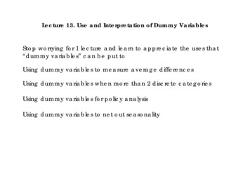
Fitting an InteractionTwo approachesLet JMP build the products for youBuild products of the dummy and numerical variablesand add these to the regression modelJMP builds this model by “crossing” the numberof households with the locationSummary of FitRegression PlotSales ( 000)250downtownmallstreet200RSquareRSquare AdjRoot Mean Square ErrorMean of ResponseObservations (or Sum Wgts)0.9876570.98086.799532176.989315Indicator Function Parameterization150100100150200Households (000)250TermInterceptHouseholds town]*Households (000)Location[mall]*Households 0.03363-0.091717Std 3DFDen9.009.009.009.009.009.00t Ratio0.467.460.481.99-0.24-0.65Mall: ŷ 7.90 0.921 Households 42.73 - 0.092 Households! ! 50.63 0.829 HouseholdsProb t 0.6538 .0001*0.64140.07820.81320.533413
Testing the InteractionFitted equation with the interaction reproducesoriginal simple regressions for each category:! ! Are the slopes really so different?Partial F testTest H0: βinteraction terms 0; not significant.E!ect TestsSourceHouseholds (000)LocationLocation*Households (000)Nparm122DF122Sum ofSquares13437.839229.35327.362F Ratio290.65072.48040.2959Prob F .0001*0.13870.7508Location is not statistically significant when theinteraction is present in the fitted model.Typical advice: Remove an interaction that is notstatistically significant.Decide status of Location after simplifying model.14
Checking AssumptionsUsual diagnostic plotsColor-coding is very helpfulHouseholds (000)Residual by Predicted PlotLocationLeverage Plot0-5-10-15100150200Sales ( 000) Predicted250250Sales ( 000)Leverage ResidualsSales ( 000)Leverage Residuals5Sales ( 000)ResidualLeverage Plot250200150100100150200Households (000)Leverage, P .0001200150100250165 170 175 180 185 190 195 200Location Leverage, P .0001Least Squares Means TableLeast squares meansLeveldowntownmallstreetLeastSq Mean172.10727193.61725165.24349Std Error3.03407652.87301653.2142985Average of response in each group at the average valueof the explanatory variableHandy comparison among groups at common value ofexplanatory variableMean195.038202.998132.93215
Another DiagnosticWhy assume that variances of the errors arethe same in each group?Slopes, intercepts may be differentWhy force all 3 groups to have the same RMSE?Plot residuals, grouped by categoryToo few to be definitive in this example (5 in each), butseem similarOneway Analysis of Residual Sales ( 000) By LocationResidualSales ( 000)50-5-10-15downtownmallstreetLocation16
PredictionUse fitted model with number of households,location to predict salesIndicator Function ParameterizationTermInterceptHouseholds 76930.86858846.863776828.373756Std 011.0011.00t Ratio2.4221.451.446.36Prob t 0.0340* .0001*0.1780 .0001*Prediction interval determined by commonestimate s2 and any extrapolation.Residual Sales ( 000)Check the normal quantileplot before rely on normality.01.05.10 .25.50 .75 .90.95.9950-5-10-1512 3 45 6Count-3-2-10123Normal Quantile Plot17
SummaryDistinguishing groups using dummy variablesRefer to JMP’s “indicator parameterization”Partial F testTest a subset of estimates, such as those associated witha categorical variableInteraction: slope depends on groupOther types of interaction, such as quadratic aredescribed in the textDiscussionWhy not fit separate regressions for each group?18
Let JMP build the products for you Build products of the dummy and numerical variables and add these to the regression model JMP builds this model by "crossing" the number of households with the location 13 100 150 200 250 Sales ( 000) 100 150 200 250 Households (000) downtown mall street Regression Plot RSquare RSquare Adj Root Mean Square .