Transcription
Regression Methods for Survey DataProfessor Ron Fricker!Naval Postgraduate School!Monterey, California!3/26/13Reading:!Lohr chapter 11!1
Goals for this Lecture! Linear regression!– Review of linear regression, including assumptions!– Coding nominal independent variables!– Running multiple regression in JMP and R! For complex sampling designs, must use R orother specialized software! Logistic regression!– Useful for binary and ordinal dependent variables!– Running logistic regression in JMP and R! For complex sampling designs, must use R orother specialized software!3/26/132
Regression in Surveys! Useful for modeling responses to surveyquestion(s) as function of external data and/orother survey data!– Sometimes easier/more efficient then highdimensional multi-way tables!– Useful for summarizing how changes in theindependent variables (the Xs) affect thedependent variable (the Y )3/26/133
Simple Linear Regression! General expression for a simple linearregression model: !Yi β0 β1xi ε i––β 0 and β1 are model parameters!ε is the error or noise term! Can think of it as modeling the expectedvalue of Y for a given or particular value of x:E (Yi xi ) β 0 β1xi!– So the result is a model of the mean of Y as alinear function of some independent variable !3/26/134
Linear Regression Assumptions ! Error terms often assumed independentobservations from a N (0, σ 2 ) distribution!Yi N ( β 0 β1 xi , σ 2 )– This encapsulates all the assumptions inherent inlinear regression:! The error terms are independent and identicallydistributed! Dependent variable is normally distributed! Hence, it is not appropriate to apply thismethodology when the Y is discrete!– So, Y can’t be based on closed-ended surveyquestions such as a 5-point Likert scale!3/26/135
Applying Linear Models to Survey Data! As a minimum the Ys must be continuous andmust be able to transform it to be symmetric!– Combinations of discrete survey data may beapproximately normally distributed!– Factor analysis and principle components may beuseful in this regard! Given some data, we will estimate theparameters with coefficients! E (Y xi ) ŷ β̂0 β̂1xiwhere ŷ is the predicted value of y3/26/136
Linear Regression withCategorical Independent Variables! Because survey data often discrete, oftenhave discrete independent variable in model!– For example, how to put “male” and “female”categories in a regression equation?!– Code them as indicator (dummy) variables! Two ways of making dummy variables:!– Male 1, female 0 !» Default in many programs !» Easy to code and interpret!– Male 1, female -1!» Default in JMP for nominal variables !» Some consider results easier to interpret! Consider a model with only gender as theindependent variable !3/26/137
Example:Calculus Grade as a Function of Gender!Regression equation:females:y 80.41 - 0.48 x 0males:y 80.41 - 0.48 x 10/1 codingCompares calc gradeto a baseline group(here, females)-1/1 codingCompares each groupto overall averageRegression equation:females: y 80.18 0.24 x1males: y 80.18 0.24 x (-1)3/26/138
How to Code k Levels! Two coding schemes: 0/1 and 1/0/-1!– Use k-1 indicator variables! E.g., three level variable: “a,” “b,”, & “c”! 0/1: use one of the levels as a baseline!Ø Var a 1 if level a, 0 otherwise!Ø Var b 1 if level b, 0 otherwise!Ø Var c – exclude as redundant (baseline)! Example:!3/26/139
How to Code k Levels (cont’d)! 1/0/-1: use the mean as a baseline!Ø Variable[a] 1 if variable a, 0 if variable b,-1 if variable c!Ø Variable[b] 1 if variable b, 0 if variable a,-1 if variable c!Ø Variable[c] – exclude as redundant! Example!3/26/1310
Fitting Simple Linear Regression Models! In JMP, can use either Analyze Fit Y by Xor Analyze Fit Model !– Fill in Y with (continuous) dependent variable !– Put X in model by highlighting and then clicking Xor “Add”!– Click “Run Model” when done! In R, use the lm() function in the basepackage!– Syntax lm(dep var indep var, data data.frame)– Best to assign results to an object and then look atresults using the summary() function!3/26/1311
Example: New Student Survey! Define a Y variable that represents thecomplete in-processing experience:!– “In-processing Total” sum(Q2a-Q2i)!3/26/1312
New Student Survey (continued)! Dependent variable looks roughly continuousand approximately normally distributed:!Normal Q-Q Plot3025101520Sample Quantiles354045Summary Statistics from JMP!-2-1012Theoretical QuantilesSummary Statistics from R! summary(new student IP total)Min. 1st Qu. MedianMean 3rd 13
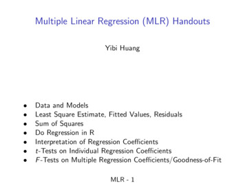
Example: Simple Linear Regressionof Total Satisfaction on School in R! model results - lm(IP total CurricNumber, data new student) summary(model results)Call:lm(formula IP total CurricNumber, data new student)Residuals:Min1Q-22.3208 Three 0/1indicators for4 schools!Estimate Std. Error t value Pr( t )(Intercept)33.5651.465 22.907 2e-16 ***CurricNumberGSEAS-4.5871.795 -2.5560.0116 *CurricNumberGSOIS-1.2441.755 -0.7090.4793CurricNumberSIGS-2.2921.909 -1.2010.2316--Signif. codes: 0 ‘***’ 0.001 ‘**’ 0.01 ‘*’ 0.05 ‘.’ 0.1 ‘ ’ 1Residual standard error: 7.027 on 151 degrees of freedom(16 observations deleted due to missingness)Multiple R-squared: 0.05347,Adjusted R-squared: 0.03466F-statistic: 2.843 on 3 and 151 DF, p-value: 0.03976Result: GSBPP students most satisfied with mean score of 33.565!GSEAS least satisfied with mean score of 33.565-4.587 28.978!3/26/1314
From Simple to Multiple Regression! Simple linear regression: One Y variable andone x variable (Yi β0 β1xi ε i )! Multiple regression: One Y variable andmultiple x variables!– Like simple regression, we’re trying to model howY depends on x!– Only now we are building models where Y maydepend on many xs!Yi β0 β1x1i β 2 x1i β k xki ε i3/26/1315
Multiple Regression in JMP(Assuming Simple Random Sampling)! In JMP, use Analyze Fit Model to domultiple regression!– Fill in Y with (continuous) dependent variable !– Put Xs in model by highlighting and then clicking“Add”! Use “Remove” to take out Xs!– Click “Run Model” when done! In R, same function and syntax as simplelinear regression, just add more terms:!– lm(dep var indep var1 indep var2 indep var3, data data.frame)3/26/1316
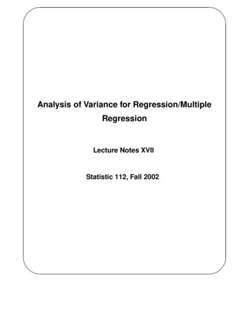
Example: RevisitingSatisfaction with In-processing (1)!GSEAS worst at in-processing?Or are CIVs and USAF least happy? Note this differs from R output because of different coding! But solution is the same: GSEAS 31.534 – 2.556 28.978!3/26/1317
Satisfaction with In-processing (2)!Or are Singaporians unhappy?3/26/13Making a new variable 18
Satisfaction with In-processing (3)! Final 0-25-3-2-10123Normal Quantile Plot3/26/1319
Equivalent Model in R(Assuming Simple Random Sampling)! summary(model results)Call:lm(formula IP total Type Student, data new student)Residuals:Min1Q-22.038 mate Std. Error t value Pr( t )(Intercept)16.5004.8103.430 0.000782Type StudentOther FORNAT16.5004.9993.301 0.001209Type StudentSingapore12.0425.0072.405 0.017400Type StudentUS Air Force7.8336.2101.261 0.209140Type StudentUS Army17.1675.1213.352 0.001017Type StudentUS Marine Corps11.7865.4542.161 0.032316Type StudentUS Navy15.5384.8713.190 0.001736--Signif. codes: 0 ‘***’ 0.001 ‘**’ 0.01 ‘*’ 0.05 ‘.’ 0.1 ‘ ’ 1***********Residual standard error: 6.803 on 148 degrees of freedom(16 observations deleted due to missingness)Multiple R-squared: 0.1306,Adjusted R-squared: 0.09539F-statistic: 3.707 on 6 and 148 DF, p-value: 0.0018383/26/1320
Now, Regression with Complex Sampling ! Use the survey package and the svyglm()function!– Don’t specify family option for linear regression!– As with other “svy” functions, must first specify thesampling design with the svydesign() functionand then call it from the svyglm() function! Open question: When fitting regressionmodels, is it necessary to account forsampling design?!– Not always clear: It may be possible with somedata to estimate relationships in the populationwithout the design and/or weights!3/26/1321
Logistic Regression! Logistic regression!– Response (Y) is binary representing event or not!– Model estimates probability of event occurrence ! pi ln β0 β1x1i β 2 x2i β k xki ε i 1 pi In surveys, useful for modeling:!– Probability respondent says “yes” (or “no”)! Can also dichotomize other questions!– Probability respondent in a (binary) class!3/26/1322
Three Numbers for the Same Idea! Probability (p)!– Example: Pr(Congress passes FY14 budget) 1/3 0.333 !– Easily interpretable – number between 0 and 1! Odds: p /(1-p)!– Example: Odds of an FY14 budget are 1/2 0.50!– Still interpretable, but not as easy as probability – anynumber 0! Log odds: ln(p/1-p)!– Very difficult to interpret – any number from to !– Log odds is often called “logit” !– In spite of interpretation difficulty, the model is very useful(and the logit can be transformed to get the probabilities)!3/26/1323
Where Logistic Regression Fits!3/26/13ContinuousCategoricalDependent or Response!Independent or Predictor ar reg.w/ dummyvariablesLogisticregressionLogistic reg.w/ dummyvariables!!!!24
Why Logistic Regression?! Some reasons:!– Estimates of p bounded between 0 and 1!– Resulting “S” curve fits many observedphenomenon!– Model follows the same general principles aslinear regression! In terms of surveys, discrete data verycommon!– If a variable is not already binary, often relativelyeasy to convert into binary result (collapseappropriately across some categories)!3/26/1325
Estimating the Parameters! β s estimated via maximum likelihood! Given estimated βs, probability is calculatedas!exp β̂0 β̂1x1i β̂ 2 x2i β̂ k xkip̂i 1 exp β̂0 β̂1x1i β̂ 2 x2i β̂ k xki(()) In JMP, after Fit Model, red triangle SaveProbability Formula!– Creates a new column containing the estimatedprobabilities, one for each observation! In R, use the predict function on an objectthat contains the output of svyglm()3/26/1326
Fitting Logistic Regression Models(Assuming Simple Random Sampling)! In JMP, fit much like multiple regression:Analyze Fit Model!– Fill in Y with nominal binary dependent variable !– Put Xs in model by highlighting and then clicking“Add”! Use “Remove” to take out Xs!– Click “Run Model” when done! In R, use the svyglm function with the optionfamily quasibinomial()3/26/1327
Example: Logistic Regression in JMP forthe New Student Survey Q1! Dichotomize Q1 into “satisfied” (4 or 5) and“not satisfied” (1, 2, or 3)! Model satisfied on Gender and Type Student!3/26/1328
Same Example in R! new student satisfied ind - as.numeric(new student X1 3) model results - glm(satisfied ind Sex Type Student, data new student, family binomial) summary(model results)Call: glm(formula satisfied ind Sex Type Student, family binomial, data new student)Deviance x1.3350Coefficients:Estimate Std. Error z value Pr( z )(Intercept)-1.33641.5411 -0.8670.386SexM1.33640.61222.1830.029 *Type StudentOther FORNAT1.70471.51511.1250.261Type StudentSingapore-0.36301.4726 -0.2470.805Type StudentUS Air Force-0.32261.9043 -0.1690.865Type StudentUS Army1.50561.56000.9650.334Type StudentUS Marine Corps2.60811.82841.4260.154Type StudentUS Navy1.95561.45651.3430.179--Signif. codes: 0 ‘***’ 0.001 ‘**’ 0.01 ‘*’ 0.05 ‘.’ 0.1 ‘ ’ 1(Dispersion parameter for binomial family taken to be 1)Null deviance: 178.83 on 161 degrees of freedomResidual deviance: 151.10 on 154 degrees of freedom(9 observations deleted due to missingness)AIC: 167.1Number of Fisher Scoring iterations: 43/26/1329
Interpreting the Output (1)! Exponentiating both sides of! pi ln β0 β1 X 1i β 2 X 2i β k X ki 1 pi pi exp ( β0 ) exp ( β1 X 1i ) exp ( β k X ki )gives!1 pi Note that the left side is the odds for the ithobservation!– A useful quantity, and one that is easy toassociate the betas to when using a 0/1 codingscheme!3/26/1330
Interpreting the Output (2)! For example, in the “baseline group” all theindicators are 0, sopi exp ( β0 )1 pi– Thus, exp ( β 0 ) is the “baseline group” odds – here,civilian female: odds exp(-1.3364) 0.26– So, the odds a female civilian is satisfied areroughly 1 to 4– In terms of probability,exp β̂00.26p̂i 0.2061 0.261 exp β̂0( )( )3/26/1331
Interpreting the Output (3)! Other groups are excursions from thebaseline using appropriate values ofindependent variables For example, consider Navy males:pi exp ( 1.3364 ) exp(1.3364) exp(1.9556) 7.071 pi– Odds male US Navy officer is satisfied are 7 to 1– In terms of probability,p̂i 3/26/13(exp β̂0 β̂ Male β̂ Navy()1 exp β̂0 β̂ Male β̂ Navy) exp (1.9556 )1 exp (1.9556 ) 0.87632
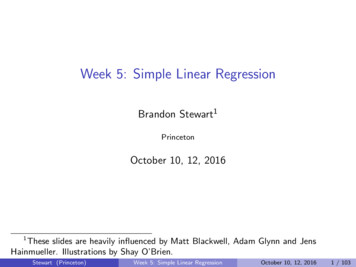
Compare Model Output to Raw Data!Coefficients:(Intercept)SexMType StudentOther FORNATType StudentSingaporeType StudentUS Air ForceType StudentUS ArmyType StudentUS Marine CorpsType StudentUS Navy3/26/13Estimate Std. Error z value Pr( z )-1.33641.5411 -0.8670.3861.33640.61222.1830.029 *1.70471.51511.1250.261-0.36301.4726 -0.2470.805-0.32261.9043 0.1541.95561.45651.3430.17933
Ordinal Logistic Regression! An extension of binary logistic regressionwhen there are k 2 dependent variablecategories!– For the ordered responses 1 j k 1, the model is! Pr(Yi j) ln α j β1 X 1i β 2 X 2i β k X ki 1 Pr(Yi j) !– Note that the betas are constant across all the js;the only difference are the alpha intercept terms! This is a proportional odds model!– In R, use polr() in the MASS library with SRSand svyolr() with complex designs!3/26/1334
An Example: New Student SurveyModeling All Q1 Likert Scale Levels! model results - polr(as.factor(X1) as.factor(Type Student), data new student) summary(model results)Call:polr(formula as.factor(X1) as.factor(Type Student), data new student)Coefficients:Value Std. Error t valueas.factor(Type Student)Other FORNAT1.46331.282 1.1416as.factor(Type Student)Singapore-0.64131.263 -0.5076as.factor(Type Student)US Air Force-0.39561.722 -0.2298as.factor(Type Student)US Army1.32111.330 0.9935as.factor(Type Student)US Marine Corps 1.71591.426 1.2032as.factor(Type Student)US Navy1.40781.238 1.1374Intercepts:ValueStd. Error1 2 -3.7123 1.39692 3 -1.6041 1.22813 4 -0.2294 1.21134 5 2.8807 1.2378t value-2.6575-1.3062-0.18942.3272Residual Deviance: 343.1792AIC: 363.1792(9 observations deleted due to missingness)3/26/1335
Interpreting the Output (1)! More complicated to understand this type ofmodel!– Most relevant are the coefficients!– Each is the estimate of how much the log-oddsincreases with a one unit change ! Can calculate the probabilities as:!Pr (Yi j ) (exp α̂ j β̂1x1i β̂ 2 x2i β̂ k xki()1 exp α̂ j β̂1x1i β̂ 2 x2i β̂ k xki)– The minus signs are correct: this is the way thepolr() function parameterizes the model!3/26/1336
Interpreting the Output (2)! So, for Navy students,!exp ( -3.7123-1.4078)Pr (Yi 1) 0.0061 exp ( -3.7123-1.4078) Similarly Pr (Yi 2 ) 0.047 , Pr (Yi 3) 0.163 ,and!Pr (Yi 4 ) 0.813 Thus, the model estimates that! 0.006,j 1! Pr (Yi j Naval Officer ) 3/26/13 0.041,j 20.116,j 30.650,j 40.187,j 537
Interpreting the Output (3)! So, for Singaporean students,!exp ( -3.7123 0.6413)Pr (Yi 1) 0.0441 exp ( -3.7123 0.6413) Similarly Pr (Yi 2 ) 0.276, Pr (Yi 3) 0.602 ,and! Pr (Yi 4 ) 0.971 Thus, the model estimates that! 0.044,j 1! Pr (Yi j Singapore Officer ) 3/26/13 0.232,j 20.326,j 30.369,j 40.029,j 538
Using R with Complex Sampling! As we’ve seen, key is the survey packageby Thomas Lumley!– See http://faculty.washington.edu/tlumley/survey/!– Other useful “svy” functions include svytable(),svyboxplot(), svyby(), svycdf(),svycoplot(), svycoxph()– Good reference text:!Lumley, T. (2010). Complex Surveys: A Guide toAnalysis using R. Wiley Series in SurveyMethodology, John Wiley and Sons.!3/26/1339
Other Software for Analyzing SurveysWith Complex Sampling Designs! Stata! SAS! SPSS! SUDAAN!!ü Not Excel or JMP!3/26/1340
What We Have Just Learned! Linear regression!– Review of linear regression, including assumptions!– Coding nominal independent variables!– Running multiple regression in JMP and R! For complex sampling designs, must use R orother specialized software! Logistic regression!– Useful for binary and ordinal dependent variables!– Running logistic regression in JMP and R! For complex sampling designs, must use R orother specialized software!3/26/1341
Multiple Regression in JMP (Assuming Simple Random Sampling)! In JMP, use Analyze Fit Model to do multiple regression! - Fill in Y with (continuous) dependent variable ! - Put Xs in model by highlighting and then clicking "Add"! Use "Remove" to take out Xs! - Click "Run Model" when done!