Transcription
GENERALIZED REGRESSIONDOE ANALYSISIN JMP PRO 12Chris Gotwalt Director of JMP Statistical R&D JMP Division, SAS Institute Clay Barker Senior Research StatisticianJMP Division, SAS InstituteCopyright 2013, SAS Institute Inc. All rightsreserved.
GENERALIZEDINTRODUCTIONREGRESSION Design of experiments (DOE) is a powerful tool for productand process improvement. JMP is well known as one of the leading software productsfor the design and analysis of experiments. JMP Pro extends modeling capabilities of JMP to moresophisticated data mining models, but is really so muchmore than that! Generalized Regression is a JMP Pro platform for linearmodels that has powerful tools for analyzing observationaldata as well as DOE data!Copyright 2013, SAS Institute Inc. All rightsreserved.
GENERALIZEDREGRESSION OLD-SCHOOL ANALYSIS OF DOEsHistorically, analysis of DOEs tends to reflect thecomputational technology of the time: Orthogonal designs - Easy to compute coefficients. Transformations - Stabilize variance with a singletransformation of the responses (log, sqrt, inverse). VIFs as a measure of multicollinear inputs. “Manual backward selection” workflow - Fit full model,remove terms with large p-values, refit model andrepeat.Copyright 2013, SAS Institute Inc. All rightsreserved.
GENERALIZED21st CENTURY DOE ANALYSIS SOFTWAREREGRESSION As computational power and user interfaces improve, better andmore direct approaches are possible: Model selection should be an integral component of theanalysis. The entire modeling process should be highly visual andinteractive. Models using non-normal distributions are a better way tohandle variance heterogeneity than transforming theresponse and then running a least squares analysis. Tradeoff analysis of different models should be quick andeasy using instantly responsive visual tools.Copyright 2013, SAS Institute Inc. All rightsreserved.
GENERALIZEDOVERVIEWREGRESSION Generalized Regression (GenReg) in JMP Pro 12 is a gamechanger in how DOEs are analyzed: One-stop shopping for analyzing DOEs since modelselection and extraction of useful information (Profilers,diagnostics, multiple comparisons) from the model are alllocated in the same place. Like having stepwise, least squares, and generalizedlinear models and logistic all in the same place, but isreally so much more! Learning a little GenReg goes a long way: Common interface for many different models! Least Sq., logistic, Poisson, quantile regression, etc. Cox PH, censored responses coming in JMP Pro 13Copyright 2013, SAS Institute Inc. All rightsreserved.
GENERALIZEDREGRESSIONTODAY’S GOALS Use case studies to demonstrate a fully modern modelselection-based approach that emphasizes interactive tools toassess the practical importance of experimental factors. Traditional approaches start with the “full” model and possiblyprune the model by removing statistically insignificant factors. We propose what amounts to a hybrid approach to analyzingDOEs that is part algorithmic, part interactive:1)2)Identify a set of plausible candidate models.Use interactive tools in JMP along with your subjectmatter knowledge to choose the best one.Copyright 2013, SAS Institute Inc. All rightsreserved.
GENERALIZEDREGRESSIONTODAY’S GOALS Demonstrate how to leverage the Solution Path plot as away to interpret the data and explore different models. Use Variable Importance in JMP Profiler to assess whichfactors are the most important predictors of theresponse.Copyright 2013, SAS Institute Inc. All rightsreserved.
GENERALIZEDREACTOR DATAREGRESSION From “Statistics For Experimenters” by Box, Hunter, andHunter. Five factor, 32 run full factorial to optimize the percentreacted in a nuclear reactor.Copyright 2013, SAS Institute Inc. All rightsreserved.
GENERALIZEDREACTOR DATAREGRESSION Right-click on the “Model” script, this brings up Fit Model,switch the personality to Generalized Regression, andclick Run.Copyright 2013, SAS Institute Inc. All rightsreserved.
GENERALIZEDREACTOR DATAREGRESSION For well-designed experiments like this one, I recommendusing Forward Selection and the AICc to find the recommendedset of factors and interactions.Copyright 2013, SAS Institute Inc. All rightsreserved.
GENERALIZEDREGRESSIONSOLUTION PATH PLOT The Solution Path (SP) is really two plots: Left: Plot of the model coefficients per step in thealgorithm. Right: Plots the AICc model-selection criteria by step. The red lines correspond to the ”Goldilocks” model thatoptimizes goodness of fit and model complexity.Copyright 2013, SAS Institute Inc. All rightsreserved.
GENERALIZEDREGRESSIONFORWARD SELECTION AND THE SOLUTION PATHThe Solution Path makes it easy to see what the modelfitting/selection algorithm is doing:1)Compute p-values for all the effects eligible to enterthe model while respecting the Effect Heredity Rule.2)Add the term with the smallest p-value to the model, fitthe new model, and calculate the models AICc (orother model-selection criteria generally).3)If there are no more terms that can be added, thenSTOP, otherwise GOTO (1).Copyright 2013, SAS Institute Inc. All rightsreserved.
GENERALIZEDREGRESSIONSELECTION CRITERIA The goal in DOE analysis is to find the model (set of maineffects and polynomial terms) that just the terms that arepredictive of the response and without the ones that donot drive the response. The we use that model forprediction, optimization, product improvement, etc. We can always improve the fit (reduce SSE) by addingmore terms to the model, regardless of whether the termis actually related to the response or not. If adding terms always improves the model, how do weknow when to stop adding terms to the model? How do wedecide which model is the best, or which ones are thegood ones?Copyright 2013, SAS Institute Inc. All rightsreserved.
GENERALIZEDREGRESSIONSELECTION CRITERIA The model ultimately used balances several considerations:1. Does that model fit the data well? (goodness of fit)2. Does the model have too many terms (modelcomplexity)3. Does the model make sense relative to our subjectmatter expertise and experience?4. What is the goal of the current experiment, factorscreening or prediction? Model selection criteria like the AICc and BIC offer guidanceon what the data says about the tradeoff of model complexityvs. goodness of fit. (1. and 2.) The practitioner uses 3. to decide add terms to the model viaforcing or choosing a particular model in the path. In screening one might tolerate more Type I errors, addingmore terms from the solution path. Prediction one may bepickier. Again, model selection criteria offer guidance.Copyright 2013, SAS Institute Inc. All rightsreserved.
GENERALIZEDREGRESSIONTHE AICc MODEL-SELECTION CRITERIA The AICc estimates the tradeoff between goodness of fitand model complexity. Experience has shown us that theAICc is a good guide to choosing models via selectingmodels with low AICc values. AICc n log(SSE/n) 2p 2p(p 1)/(n-p-1) constant. As Forward Selection adds terms to the model, the SSEgoes down (decreasing AICc), but increasing p serves toincrease the AICc. “Model Selection and Multimodel Inference” by Burnhamand Anderson is an excellent book on how to use theAICc.Copyright 2013, SAS Institute Inc. All rightsreserved.
GENERALIZEDREGRESSIONINTERPRETING THE SOLUTION PATH Usually, early in FS the AICc decreases, reaches itslowest point, and then climbs up as FS ends at the fullmodel with all the possible terms in it. Models left of the red line are “too simple,” models to theright are “too complicated.” The red line is the “Goldilocks” model and has the “best”tradeoff of goodness of fit to model complexity. “Green Zone” models are strongly consistent with the bestmodel. Green Zone Best AICc 4. “Yellow Zone” models are strongly consistent with the bestmodel. Yellow Zone Best AICc 10.Copyright 2013, SAS Institute Inc. All rightsreserved.
GENERALIZEDREGRESSIONTHE BIC MODEL-SELECTION CRITERIA The BIC is another popular criteria which is used similarlyto the AICc. BIC n log(SSE/n) p log(n) constant. BIC tends to select models with more terms than the AICcwith small datasets. I use BIC over AIC sometimes inscreening situations.Copyright 2013, SAS Institute Inc. All rightsreserved.
GENERALIZEDREGRESSIONUSING THE SOLUTION PATH FOR INTERPRETATIONCopyright 2013, SAS Institute Inc. All rightsreserved.
GENERALIZEDREGRESSIONINTERPRETING THE SOLUTION PATH The parameter paths are selectable and are dynamicallyconnected to the report. Move the black arrow to change the model being viewed.The entire report, including all graphics and tables,updates immediately. Blue lines are coefficients in the current model; black onesare zero-valued coefficients not in the current model. The parameter paths show strength and direction of therelationship with the response. The shape of the lines gives interesting information aboutthe design. In this case, the lines are constant, whichmeans the design is orthogonal.Copyright 2013, SAS Institute Inc. All rightsreserved.
GENERALIZEDREGRESSIONINTERPRETING THE SOLUTION PATH We see a range of models (Steps 5-9) within the greenand yellow zones. These models have good support fromthe data. There is almost no difference between Step 6 (the bestmodel) and Step 5, which differ by Catalyst*Concentration.Although it is marginally significant, we might considerdropping it from the model. Interactively changing the model in the zones incombination with the Profiler and Actual by Predicted plotsdoes not show big changes. A combination of goodness of fit, sensible modelparsimony, and subject matter knowledge should be usedto determine the final model.Copyright 2013, SAS Institute Inc. All rightsreserved.
GENERALIZEDREGRESSIONNON-NORMAL DISTRIBUTIONS Non-Normal distributions are common, but are not part of thetraditional DOE training. They happen often when the response is strictly positive, asuccess/failure binary, a count. Greater variation for larger values of the response is often bestexplained by non-normality. The old-school approach would be to transform the response. A modern, unified approach is to fit non-normal distributionsand choose one based on the model selection criteria andyour subject matter knowledge.This is just like how we do variable selection!Copyright 2013, SAS Institute Inc. All rightsreserved.
GENERALIZEDREGRESSIONNON-NORMAL DISTRIBUTIONS Cauchy – Outliers Binomial – Binary andnSuccess out of nTrials. Poisson – Count data Beta – Proportions (0,1) Gamma, Exponential - (0, ) ZI – “Zero-Inflated” Beta. Binom, Neg. Poisson –“Overdispersed” count data.Copyright 2013, SAS Institute Inc. All rightsreserved.
GENERALIZEDREGRESSIONBETA MODEL FOR THE REACTOR DATA Reactor’s response is a proportion. Predictions outside(0,1) are meaningless. The Beta distribution is a possible alternative to theNormal distribution. The best Beta AICc is -100, vs. -115 for the Normal. TheNormal Predictions stay in (0,1) range. I would stay withthe Normal, but it is easy and worthwhile to take a look.Copyright 2013, SAS Institute Inc. All rightsreserved.
GENERALIZEDREGRESSIONTHE PROFILER The Profiler is an extremely useful tool for extractinginformation about a model. It shows traces (profiles) of the prediction formula wrteach input variable, holding the other ones constant.Copyright 2013, SAS Institute Inc. All rightsreserved.
GENERALIZEDREGRESSION THE PROFILERThe Profiler is where one: Extracts predictions and prediction intervals from a model. Optimizes a model, possibly with constraints. Assess variable importance.Copyright 2013, SAS Institute Inc. All rightsreserved.
GENERALIZEDREGRESSIONASSESSING VARIABLE IMPORTANCE What are the most important variables in our model? There are several related statistical tools for this: Sums of Squares: How much variation in the data isexplained by a variable (or interaction, squared term)? P-Value: How likely is that you would see a largercoefficient than the one observed if the “true” one iszero?Neither of these tools directly tells us what are the mostimportant variables in the model.Copyright 2013, SAS Institute Inc. All rightsreserved.
GENERALIZEDREGRESSIONASSESSING VARIABLE IMPORTANCE Example: A regression coefficient can be highly significantwith p .0001 but still be very small in impact on the functionthat has been fit to the data (small coefficient, very smallstandard error). Another problem is that measures of variable importancetend to reflect the structure of the model and often don’tgeneralize to other models. A method like sums of squares works well for linear models,but is not intended for binary response models, PLS models,or Neural models.Copyright 2013, SAS Institute Inc. All rightsreserved.
GENERALIZEDREGRESSIONSOBOL’S SENSITIVITY INDICES Sobol’s Sensitivity Indices are a general method for quantifyingthe amount of variability of a general function due to each of theinputs. Based on a decomposition of a function with regard to aprobability density, 𝜇(𝑥1 , 𝑥2 , , 𝑥𝑘 ).𝑘𝑓 𝑋 𝑓0 𝑓𝑖 𝑥𝑖 𝑖 1 𝑘𝑓𝑖𝑗 𝑥𝑖 , 𝑥𝑗 𝑓12 𝑘 (𝑥1 , 𝑥2 , , 𝑥𝑘 )𝑖 𝑗The functions, 𝑓𝑖 , 𝑓𝑖𝑗 , etc. are the marginal models and areorthogonal wrt probability measure 𝜇(𝑥1 , 𝑥2 , , 𝑥𝑘 ).Copyright 2013, SAS Institute Inc. All rightsreserved.
GENERALIZED SOBOL’S SENSITIVITY INDICESREGRESSION𝑘𝑖 1 𝑓𝑖 𝑓 𝑋 𝑓0 Where, for example:𝑓0 𝑓1 𝑥𝑖 𝑘𝑖 𝑗 𝑓𝑖𝑗𝑥𝑖 , 𝑥𝑗 𝑓12 𝑘 (𝑥1 , 𝑥2 , , 𝑥𝑘 )𝑓 𝑥1 , , 𝑥𝑘 𝑑𝜇 𝑥1 , 𝑥2 , , 𝑥𝑘 𝐸(𝑓(𝑥1 , , 𝑥𝑘 ))(overall average)𝑓 𝑥1 , 𝑥2 , , 𝑥𝑘 𝑑𝜇 𝑥2 , , 𝑥𝑘 𝑓0 𝐸(𝑓(𝑥1 , , 𝑥𝑘 ) 𝑥1 ) 𝑓0(marginal 𝑥1 main effect)𝑓12 𝑓 𝑥1 , 𝑥2 , , 𝑥𝑘 𝑑𝜇 𝑥3 , , 𝑥𝑘 𝑓0 𝑓1 𝑥1 𝑓2 𝑥2 𝐸(𝑓(𝑥1 , , 𝑥𝑘 ) 𝑥3 , , 𝑥𝑘 ) 𝑓0 𝑓1 𝑥1 𝑓2 𝑥2(marginal 𝑥1 𝑥2 interaction effect)Copyright 2013, SAS Institute Inc. All rightsreserved.
GENERALIZEDREGRESSIONMAIN EFFECT IMPORTANCES The idea is that the variability in the function can be uniquelydecomposed into sums of squares attributable to each ofthese main effects and interaction terms. For example, 𝑆𝑆𝑄𝑖 𝑆𝑆𝑄𝑡𝑜𝑡𝑎𝑙 ( 𝑓 𝑥1 , , 𝑥𝑘 𝑓0 )2 𝑑𝜇 𝑥1 , , 𝑥𝑘 𝑉𝑎𝑟(𝑓 𝑥1 , , 𝑥𝑘 ) 𝑆𝑖 𝑓𝑖2 𝑥𝑖 𝑑𝜇 𝑥𝑖 𝑉𝑎𝑟( (𝐸( 𝑓𝑖 (𝑥𝑖 ) 𝑥𝑖 ))𝑆𝑆𝑖𝑆𝑆𝑡𝑜𝑡𝑎𝑙 𝑉𝑎𝑟( (𝐸( 𝑓𝑖 (𝑥𝑖 ) 𝑥𝑖 ))/𝑉𝑎𝑟(𝑓 𝑥1 , 𝑥2 , , 𝑥𝑘 )is the proportion of the variability due to 𝑥𝑖 acting alone. We call this the main effect importance of 𝑥𝑖 . We can similarly define interaction effect importances of any order.Copyright 2013, SAS Institute Inc. All rightsreserved.
GENERALIZEDREGRESSIONTOTAL EFFECT IMPORTANCES We measure the total impact of a variable by calculating theloss of variation that results from integrating it out: 𝑓 1 2𝑆𝑆𝑄 1 𝑓 1𝑥2 , , 𝑥𝑘 𝑑𝜇 𝑥2 , , 𝑥𝑘 𝑉𝑎𝑟(𝐸(𝑓 𝑥1 , , 𝑥𝑘 𝑓 𝑥2 , , 𝑥𝑘 )) 𝑓 𝑥1 , , 𝑥𝑘 𝑑𝜇 𝑥1 𝑓0 𝐸(𝑓 𝑥1 , , 𝑥𝑘 𝑓 𝑥2 , , 𝑥𝑘 )𝑆 1 (𝑆𝑆𝑄𝑡𝑜𝑡𝑎𝑙 𝑆𝑆𝑄 1 ) / 𝑆𝑆𝑄𝑡𝑜𝑡𝑎𝑙 1 𝑉𝑎𝑟(𝐸(𝑓 𝑥1 , , 𝑥𝑘 𝑓 𝑥2 , , 𝑥𝑘 ))/𝑉𝑎𝑟(𝑓 𝑥1 , 𝑥2 , , 𝑥𝑘is the proportion of the variability lost due to integrating 𝑥1 out. 𝑆 1 implicitly takes into consideration the main effect of 𝑥1 andall of its higher order interactions!We call this the total effect importance of 𝑥𝑖Copyright 2013, SAS Institute Inc. All rightsreserved.
GENERALIZEDREGRESSIONEFFECT IMPORTANCES One of the great things about these importances is that theymake very few assumptions about function. The same technique can be applied to linear models,response surface models, logistic models, neural networks,PLS models, tree-based models, and model averagedmodels! Although there is quite a bit of math behind the scenes, theresults are easy to use and interpret.Copyright 2013, SAS Institute Inc. All rightsreserved.
GENERALIZEDREGRESSIONEFFECT IMPORTANCE CALCULATIONS JMP uses Monte Carlo (until the standard error is 1% for allindices) to compute the integrals. There are four options for the Monte Carlo distribution: Independent Uniform Good for DOEs without constraints. Independent Resampled (from the data) Fast for observational data, ignores multicollinearity. Dependent Resampled Slower, but takes into account multicollinearity. Linearly Constrained Inputs Uniform over linearly constrained region, only forDOEs with constraints (e.g., mixture designs),prevents extrapolation out of design region.Copyright 2013, SAS Institute Inc. All rightsreserved.
GENERALIZEDREGRESSIONNITROGEN OXIDE RSM Nitrogen Oxides (NOx) are toxic greenhouse gases thatare common by-products of burning organic compounds. An experiment was done on an industrial burner tocontrol the amount of NOx it created. A 32 run I-Optimal RSM design was created with 7continuous factors: Hydrogen Fraction in primary fuel Air/Fuel Ratio Lance Position X Lance Position Y Secondary Fuel Fraction Dispersant Ethanol Percentage in primary fuelCopyright 2013, SAS Institute Inc. All rightsreserved.
GENERALIZEDREGRESSIONNITROGEN OXIDE RSMCopyright 2013, SAS Institute Inc. All rightsreserved.
GENERALIZEDLIMIT OF DETECTION DATAREGRESSION In many biological and chemical experiments, there is asmallest reading below which a reading is consideredinaccurate. This is called a lower limit of detection (LOD)on the response. A simple approach is to enter zeros for the readings at orbelow the LOD. This leads to flawed, biased results. The better way to do the analysis is to use censoring. A censored observation is one that we only observe tobe within a certain (possibly infinite) range.Copyright 2013, SAS Institute Inc. All rightsreserved.
GENERALIZEDCENSORED DATAREGRESSION There are three types of censoring: right, interval, andleft censoring. Right censoring is very common in engineering reliabilityand in clinical studies where the response is the time toan event. For example, if a patient is in a 30-day study thatevaluates a medicine that prevents migraines, and thestudy ends before the patient’s next migraine, then therecording would be a observation that is censored at 30days. All we know is that the time until the next migrainewas longer than 30 days, which should be reflected in aproper analysis.Copyright 2013, SAS Institute Inc. All rightsreserved.
GENERALIZEDLIMIT OF DETECTION DATAREGRESSION LOD data is left censored: If a measurement comes in ator below the LOD, all we know is that the actual value issomewhere between the lower detection limit and zero. Typically LOD data is strictly positive. This means thatthe data should be analyzed with a non-Gaussiandistribution to avoid negative values predictions andvariance heterogeneity. Analyzing LOD data in JMP is simple, you just have tohave the response saved properly.Copyright 2013, SAS Institute Inc. All rightsreserved.
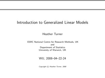
GENERALIZEDREPRESENTING LIMIT OF DETECTION DATA IN JMPREGRESSION To represent LOD data in JMP, you need two responsecolumns: a low value and a high value. The two columns are the same for values above theLOD. Data below the LOD have a missing low value and ahigh value equal to the LOD.Copyright 2013, SAS Institute Inc. All rightsreserved.
GENERALIZEDLIMIT OF DETECTION DATAREGRESSION Rows 1, 2, and 5 are above the LOD, while rows 3 and 4were at or below the LOD.Copyright 2013, SAS Institute Inc. All rightsreserved.
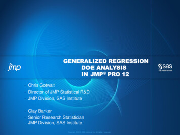
GENERALIZEDMETACRATE DOEREGRESSION Researchers wanted to optimize determination of apesticide (Metacrate) from water using Dichloromethaneand Methanol as a dispersive and a solvent. They created a 32 run I Optimal design in JMP usingDichloromethane, Methanol, and Water Sample Volumeas inputs. Four of the 32 observations were below the LOD of 1.0.Copyright 2013, SAS Institute Inc. All rightsreserved.
GENERALIZEDMETACRATE DOEREGRESSIONCopyright 2013, SAS Institute Inc. All rightsreserved.
JMP is well known as one of the leading software products for the design and analysis of experiments. JMP Pro extends modeling capabilities of JMP to more sophisticated data mining models, but is really so much more than that! Generalized Regression is a JMP Pro platform for linear models that has powerful tools for analyzing .