Transcription
TRADING VOLUME AND SERIAL CORRELATION INSTOCK RETURNS*This paper investigates the relationship between aggregate stock markettrading volume and the serial correlation of daily stock returns. For both stockindexes and individual large stocks, the first-order daily return autocorrelationtends to decline with volume. The paper explains this phenomenon using a model inwhich risk-averse "market makers" accommodate buying or selling pressure from"liquidity" or "noninformational" traders. Changing expected stock returns reward market makers for playing this role. The model implies that a stock pricedecline on a high-volume day is more likely than a stock price decline on alow-volume day to be associated with an increase in the expected stock return.There is now considerable evidence that the expected returnon the aggregate stock market varies through time. One interpretation of this fact is that it results from the interaction betweendifferent groups of investors. Suppose that some investors,"liquidity" or more generally "noninformational" traders, desireto sell stock for exogenous reasons. Other investors are risk-averseutility maximizers; they are willing to accommodate the sellingpressure, but they demand a reward in the form of a lower stockprice and a higher expected stock return. If these investorsaccommodate the fluctuations in noninformational traders' demand for stock, then they can be thought of as "market makers" inthe sense of Grossman and Miller [1988], even though they mayhold positions for relatively long periods of time and may not bespecialists on the exchange. lIt is hard to test this view of the stock market using data onstock returns alone, because very different models can have similar*We thank J. Harold Mulherin and Mason Gerety for providing data on dailyNYSE volume, G. William Schwert for providing daily stock return data, MartinLettau for correcting an error in the theoretical model, Ludger Hentschel for ableresearch assistance throughout this project, and four anonymous referees andseminar articipants a t Princeton University and the 1991 NBER SummerInstitute for helpful comments. Campbell acknowledges financial support from theNational Science Foundation and the Sloan Foundation. Wang acknowledgessupport from the Nanyang Technological University Career Development AssistantProfessorship a t the Sloan School of Management.1. See also Campbell and Kyle 119931; De Long, Shleifer, Summers, andWaldmann 11989, 19901;Shiller 119841;Wang [1993a, 1993131;and others.o 1993 by the President and Fellows of Harvard College and the Massachusetts Institute ofTechnology.The Quarterly Journal of Economics, November 1993
906QUARTERLY JOURNAL OF ECONOMICSimplications for the time-series behavior of returns. In this paperwe use data on stock market trading volume to help solve thisidentification problem. The simple intuition underlying our work isas follows. Suppose that one observes a fall in stock prices. Thiscould be due to public information that has caused all investors toreduce their valuation of the stock market, or it could be due toexogenous selling pressure by noninformational traders. In theformer case, there is no reason why the expected return on thestock market should have changed. In the latter case, marketmakers buying stock will require a higher expected return, so therewill tend to be price increases on subsequent days. The two casescan be distinguished by looking at trading volume. If publicinformation has arrived, there is no reason to expect a high volumeof trade, whereas selling pressure by noninformational tradersmust reveal itself in unusual volume. Thus, the model withheterogeneous investors suggests that price changes accompaniedby high volume will tend to be reversed; this will be less true ofprice changes on days with low volume.Shifts in the demand for stock by noninformational traderscan occur at low frequencies or at high frequencies. Daily tradingvolume is a signal for high frequency shifts in demand. Changes indemand that occur slowly through time are harder to detect usingvolume data because there are trends in volume associated withother phenomena such as the deregulation of commissions and thegrowth of institutional trading. We therefore focus on daily tradingvolume and the serial correlation of daily returns on stock indexesand individual stocks. Daily index autocorrelations are predominantly positive [Conrad and Kaul, 1988; Lo and MacKinlay, 19881,but our theory predicts that they will be less positive on highvolume days.The literature on stock market trading volume is extensive,but is mostly concerned with the relationship between volume andthe volatility of stock returns. Numerous papers have documentedthe fact that high stock market volume is associated with volatilereturns; October 19, 1987, is only the best known example of apervasive p h e n m e n o nIt. has also been noted that volume tendsto be higher when stock prices are increasing than when prices arefalling.2. See Gallant, Rossi, and Tauchen [1992];Harris [19871; Jain and Joh [19881;Jones, Kaul, and Lipson [19911; Mulherin and Gerety [19891; Tauchen and Pitts[1983]; and the survey in Karpoff [19871. Larnoureux and Lastrapes [I9901 ar ethat serial correlation in volume accounts for the serial correlation in volaticywhich is often described using ARCH models.
VOLUME AND SERIAL CORRELATION IN STOCK RETURNS907In contrast, there is almost no work relating the serialcorrelation of stock returns to the level of volume. One exception isMorse [1980], who studies the serial correlation of returns inhigh-volume periods for 50 individual securities. He finds thathigh-volume periods tend to have positively autocorrelated returns, but he does not compare high-volume with low-volumeperiod . Several recent papers study serial correlation in relationto volatility: LeBaron [1992al and Sentana and Wadhwani [19921,for example, show that the autocorrelations of daily stock returnschange with the variance of returns. Below, we compare the effectsof volume and volatility on stock return autocorrelations.The organization of our paper is as follows. In Section I1 weconduct a preliminary exploration of the relation between volume,volatility, and the serial correlation of stock returns. In Section I11we present a theoretical model of stock returns and tradingvolume. In Section IV we show that the model can generateautocorrelation patterns similar to those found in the actual data.We use both approximate analytical methods and numerical simulation methods to make this point. Section V concludes.A. Measurement IssuesThe main return series used in this paper is the daily return ona value-weighted index of stocks traded on the New York StockExchange and American Stock Exchange, measured by the Centerfor Research in Security Prices (CRSP) at the University ofChicago over the period 7/3/62 through 12/30/88. Results withdaily data over this period are likely to be dominated by a fewobservations around the stock market crash of October 19, 1987.For this reason, the main sample period we use in this paper is ashorter period running from 7/3/62 through 9130187 (1962-1987for short, or sample A). We break this period into two subsamples:7/3/62 through 12/31/74 (1962-1974 for short, or sample B),which is the first half of the shorter sample and which excludes the3. Some other papers have come to our attention since the first draft of thispaper was written. Duffee [I9921 studies the relation between serial correlation andtradingvolume in aggregate monthly data, while LeBaron [1992bl uses nonparametric methods to characterize the aggregate daily relation more accurately. Conrad,Hameed, and Niden [I9921 study the relation between individual stocks' returnautocorrelations and the tradingvolume in those stocks.
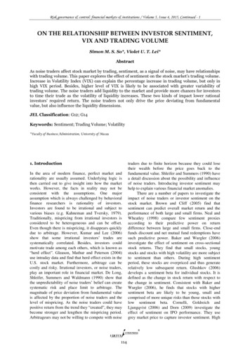
908QUARTERLY JOURNAL OF ECONOMICSperiod of flexible commissions on the New York Stock Exchange;and 1/2/75 through 9130187 (1975-1987 for short, or sample C),which is the remainder of the shorter sample period. Finally, weuse the complete data set through the end of 1988 in order to seewhether the extreme movements of price and volume in late 1987strengthen or weaken the results we obtain in our other samples.We call this long sample 1962-1988 for short, or sample D.We also study the behavior of some other stock return series.For the period before CRSP daily data begin, Schwert [I9901 hasconstructed daily returns on an index comparable to the Standardand Poors 500. We use this series over the period 112126-6/29/62.The behavior of large stocks is of particular interest, since measured returns on these stocks are unlikely to be affected bynonsynchronous trading. The Dow Jones Industrial Average is thebest known large stock price index, and so we study its changesover the period 1962-1988. Individual stock returns also provideuseful evidence robust to nonosynchronous trading, so we studythe returns on 32 large stocks that were traded throughout the1962-1988 period and were among the 100 largest stocks on both7/2/62 and 12/30/88.4Stock market trading volume data were kindly provided to usby J. Harold Mulherin and Mason S. Gerety. These researcherscollected data from The Wall Street Journal and Barron's on thenumber of shares traded daily on the New York Stock Exchangefrom 1900 through 1988. They also collected data on the number ofshares outstanding on the New York Stock Exchange. For adetailed description of their data, see Mulherin and Gerety [19891.The ratio of the number of shares traded to the number ofshares outstanding is known as turnover, or sometimes as relativevolume. Turnover is used as the volume measure in most previousstudies (for example, Jain and Joh [I9881 and Mulherin and Gerety[19891). Since the number of shares outstanding and the number ofshares traded have both grown steadily over time, the use ofturnover helps to reduce the low-frequency variation in the series.It does not eliminate it completely, however, as can be seen fromthe plot of the series presented in Figure I. Turnover has anupward trend in the late 1960s and in the period between the4. The 32 stocks are American Home Products, AT&T, Amoco, Caterpillar,Chevron, Coca Cola, Commonwealth Edison, Dow Chemical, Du Pont, EastmanKodak, Exxon, Ford, GTE, General Electric, General Motors, ITT, Imperial Oil,IBM, Merck, 3M, Mobil, Pacific Gas and Electric, Pfizer, Procter and Gamble, RJRNabisco, Royal Dutch Petroleum, SCE, Sears Roebuck, Southern, Texaco, USX, andWestinghouse.
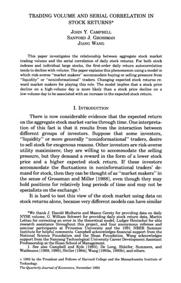
VOLUME AND SERIAL CORRELATION IN STOCK RETURNS909R a w TurnoverDateFIGUREILevel of Stock Market Turnover, 1960-1988elimination of fixed commissions in 1975 and the stock marketcrash of 1987. The growth of turnover in the 1980s may be due inpart to technological innovations that have lowered transactionscosts. In addition, the variance of turnover seems to increase withits level during the 1980s.In our empirical work, we want to work with stationary timeseries. When we relate our empirical results to our theoreticalmodel, we want to measure trading volume relative to the capacityof the market to absorb volume. For both these reasons we wish toremove the low-frequency variations from the level and variance ofthe turnover series. To remove low-frequency variations from thevariance, we measure turnover in logs rather than in absoluteunits. To detrend the log turnover series, we subtract a one-yearbackward moving average of log turnover. This gives a triangularmoving average of turnover growth rates, similar to the geometrically declining average of turnover growth rates used by Schwert[I9891 to explain stock return volatility. We explore some alternative detrending procedures below.Our detrended volume measure is plotted in Figure 11. Thefigure shows no trends in mean or variance, but it does showconsiderable persistence. The first daily autocorrelation of detrended volume is about 0.7, and the fifth daily autocorrelation is
910QUARTERLY JOURNAL OF ECONOMICSD e v i a t i o n s f r o m 1 y r MA of Log T u r n o v e r.--.'4IDateFIGUREI1Detrended Log Turnover, 1960-1988still about 0.5. The standard deviation of the series is close to 0.25;all these moments are stable across subsamples.We also need a measure of stock return volatility. We take theconditional variance series estimated by Campbell and Hentschel[I9921 using daily return data over the period 1926-1988. Campbell and Hentschel used a quadratic generalized autoregressiveheteroskedasticity (QGARCH) model with one autoregressive term,two moving average terms, and a mean return assumed to changein proportion to volatility. The QGARCH model is very similar tothe standard GARCH model of changing volatility, but it allowsnegative returns to increase volatility more than positive returnsdo.B. Forecasting Returns from Lagged Returns, Volatility, a n dVolumeTable I summarizes the evidence on the first daily autocorrelation of the value-weighted index return. For each of our foursample periods, the table reports the autocorrelation with aheteroskedasticity-consistent standard error, and the R2 statisticfor a regression of the one-day-ahead return on a constant and thereturn. This statistic, which we write as R2(1) in the table, is justthe square of the autocorrelation. The remarkable fact is that the
VOLUME AND SERIAL CORRELATION IN STOCK RETURNS(1)(2)911TABLE ITHE FIRSTAUTOCORRELATIONOF STOCKRETURNSrt l cu Prtrt l a (Z: l P,Di)rtSample periodautocorrelation exceeds 0.15 in every sample period; it is about 0.2over the full sample and nearly 0.3 in the 1962-1974 period.Table I also shows the improvement in R 2 that can be obtainedby allowing the first autocorrelation to vary with the day of theweek. A regression of the one-day-ahead return on the currentreturn interacted with five day-of-the-week dummies has an R 2statistic, labeled R 2 ( 2 )in the table, that is at least 0.5 percentagepoints larger than the R 2 of the basic regression. The increase in R 2is even greater in the 1962-1988 period, but much of this is due tothe single week of the stock market crash. The day-of-the-weekdummies are significant enough that we include them in all oursubsequent regressions.Table I1 looks at the relationship between volume and the firstautocorrelation of the value-weighted index return. We regress theone-day-ahead stock return on the current stock return interactednot only with day-of-the-week dummies but also with volume.Alternatively, we interact the current return with dummies andwith estimated conditional variance. Finally, we report a regression in which the current return is interacted with dummies,conditional variance, volume, and volume squared. The last ofthese variables is included to capture any nonlinearity that mayexist in the relation between volume and autocorrelation.Panel A of Table I1 uses the sample period 1962-1987. Overthis period Table I showed that 5.7 percent of the variance of theone-day-ahead value-weighted index return can be explained by a
912QUARTERLY JOURNAL OF ECONOMICSTABLE I1VOLUME,VOLATILITY,AND THE FIRSTAUTOCORRELATIONr t l cu ( I L 1 PiDi ylVt y z f 2 y3(1000uf2))rt-Sample periodand specification-Y1Yz(s.e.1(s.e.1Y'3(s.e.1R2A: 713162-9130187VolumeVolatilityVolume and volatilityB: 713162-12131174VolumeVolatilityVolume and volatilityC: 112175-9130187VolumeVolatilityVolume and volatilityD: 713162-12130188VolumeVolatilityVolume and volatilityregression on current return interacted with day-of-the-weekdummies. The first row of panel A shows that this R2 statistic canbe increased to 6.5 percentage points by interacting the regressorwith dummies and detrended trading volume. The coefficient onthe product of volume and the stock return is -0.33 with aheteroskedasticity-consistent standard error of 0.06. This is economically as well as statistically significant. The standard deviation of detrended volume is about 0.25. Thus, as volume movesfrom two standard deviations below the mean to two standarddeviations above, the first-order autocorrelation of the stock returnis reduced by about 0.3.
VOLUME AND SERIAL CORRELATION IN STOCK RETURNS913These strong results for volume are not matched by ourvolatility measure. When volume is excluded from the regression,volatility enters negatively, but it is statistically and economicallyinsignificant. When volume and volume squared appear in theregression, volatility enters positively but is again insignificant.The quadratic term on volume is positive and not quite significantat the 5 percent level. Thus, in panel A there is only weak evidencefor any specification more complicated than the linear volumeregression reported in the second row.In panels B and C of Table 11, we break the 1962-1987 periodinto subsamples 1962-1974 and 1975-1987. The strongest resultscome from the earlier subsample 1962-1974. In this period theaverage first-order autocorrelation of the stock return is almost0.3, and a regression of the one-day-ahead return on the currentreturn interacted with day-of-the-week dummies gives an R2statistic of 8.4 percent. This can be increased by more than apercentage point by taking account of a linear relationship betweenthe autocorrelation and trading volume. Once again volatility andquadratic volume terms add little. In the later subsample, 19751987, the first-order autocorrelation is much smaller on average.Volume raises the regression R2 from 4.3 percent only to 4.6percent, although the linear volume term is still statisticallysignificant with a t-statistic of 2.9. In this period there is a strongernegative relationship between volatility and autocorrelation, although volume is still slightly superior to volatility when both areincluded in the regression.Finally, in panel D of Table I1 we ask whether the addition ofthe stock market crash period to the sample weakens or reinforcesour results. It turns out that the most recent data weaken the effectof volume on the first-order autocorrelation of returns. Even in the1962-1988 period, however, volume remains significant at the 5percent level. We note also that the 1962-1988 period is the onlyone for which day-of-the-week dummies make a major difference tothe results. When these dummies are excluded, the volume effectbecomes much stronger in the 1962-1988 period than in the1962-1987 period. This is because the stock price reversals of theweek of October 19, 1987, are captured by day-of-the-week dummies when these are included, or by volume when dummies areomitted.Table I11 has exactly the same structure as Table I, but nowthe dependent variable is the two-day-ahead stock return so thetable describes the second-order autocorrelation of the return. The
9 14(1)(2)QUARTERLY J O U R N U OF ECONOMICSTABLE I11THE SECONDAUTOCORRELATIONOF STOCKRETURNSrt z cu prtrt z a (Zf l PiDi)rtPSample period(s.e.1R2(1)R2(2)average second-order autocorrelation is small and statisticallyinsignificant in every sample period. Even when day-of-the-weekdummies are interacted with the current return, the R2 statistic ofthe regression is less than 1.5 percent.Table IV, which has the same structure as Table 11, showssome evidence for volume effects on the second autocorrelation.However, the evidence is much weaker than that for volume effectson the first autocorrelation. Over the 1962-1987 sample period(panel A) we find that volume enters the regression significantlyonly when it is included in quadratic form. The linear coefficient is-0.23 with a standard error of 0.08, while the quadratic coefficientis 0.55 with a standard error of 0.15. These coefficients imply thatthe second-order autocorrelation falls with volume until volumereaches 0.2, about two-thirds of a standard deviation above itsmean. At higher levels of volume the positive quadratic termdominates, and the autocorrelation starts to increase again. Looking at subsamples in panels B and C, we find that the evidence forvolume effects on the second autocorrelation comes entirely fromthe 1962-1974 period. Finally, in panel D we see that the additionof the stock market crash period leads to stronger evidence for avolume effect on the second autocorrelation.One might ask whether higher-order autocorrelations alsochange with trading volume. As a crude way to answer thisquestion without having to look at each autocorrelation individu-
VOLUME AND SERIAL CORRELATION I N STOCK RETURNS915TABLE IVAND THE SECONDVOLUME,VOLATILITY,AUTOCORRELATIONrt z a (ZL1 PiDi ylVt yzV; y3(1000u;))rtSample periodand 60)VolatilityVolume and volatilityB: 11VolatilityVolume and volatilityC: 112175-9130187Volume-0.390(0.113)1.149(0.345)D: 004-0.178(0.089)0.016VolatilityVolume and volatility0.0090.074(0.069)VolatilityVolume and .007(0.105)0.0110.072(0.102)0.019ally, we have run regressions of stock returns on moving averagesof past stock returns and on moving averages of past stock returnsinteracted with trading volume. Regressions of this sort (where thelags in the moving averages run from 1 to 5 or from 2 to 6) yieldresults similar to those reported in Tables I1 and IV, withsomewhat reduced statistical significance. This suggests that themain volume effects are in the first couple of autocorrelations, butthat there are at least no offsetting effects in higher autocorrelations out to lags 5 or 6.
QUARTERLY JOURNAL O F ECONOMICSTABLE VVOLUME,VOLATILITY,AND THE FIRST AUTOCORRELATION:ALTERNATIVEVOLUMEMEASURESr t (2: 1P,Di y Vt yzMAVt ys(Vt MAVt))rtSample period andspecificationA: 713162-9130187Detrended tal volumeDetrended andtrend volumeB:713162-12131174Detrended volume-0.156(0.028)-0.313(0.061)-0.090(0.037)C: 112175-9130187Detrended volume-0.417(0.108)0.095D:713162-12130188Detrended .073)-0.090(0.046)-0.169(0.080)0.062Total volumeDetrended andtrend volume-0.227(0.081)0.292(0.141)Total volumeDetrended andtrend volume0.0640.066-0.445(0.114)Total volumeDetrended andtrend 630.064C. Alternative Volume and Volatility MeasuresSo far we have worked exclusively with detrended volume. It isnatural to ask whether similar results could be achieved withoutdetrending. To answer this, in Table V we run similar regressionsto those in Table 11, but using total volume instead of detrendedvolume. We also run regressions including both the detrendedseries and the trend. The general pattern is that detrended volumehas superior explanatory power to total volume, although this isnot true in 1975-1987. When both detrended and trend volume are
VOLUME AND SERIAL CORRELATION IN STOCK RETURNS917included, the coefficient on detrended volume is always negativeand significant, whereas the coefficient on the trend switches signfrom positive in 1962-1974 to negative in 1975-1987.In an earlier version of this paper, we also used an unobservedcomponents model to stochastically detrend volume. The resultingseries was much less persistent than the detrended series usedhere, having a positive first-order autocorrelation and than a seriesof negative higher-order autocorrelations. The stochastically detrended volume series gave results similar to but systematicallyweaker than those in Table II.5 This can be interpreted in terms ofour theoretical expectation that the serial correlation of stockreturns declines when volume increases relative to the ability ofmarket makers to absorb volume. A one-year backward movingaverage of past volume, which reacts sluggishly to changes involume, seems to be a better measure of market making capacitythan an estimated random walk component from an unobservedcomponents model, which reads very quickly to changes in v01ume. To check the robustness of this finding, we have also triedmeasuring volume as the deviations of log turnover from threemonth and five-year backward moving averages. Both these alternative moving average measures gave results similar to thosereported in Table 11. Thus, it seems to be important to measurevolume relative to a slowly adjusting trend, but the exact details oftrend construction are not crucial.The results reported above also use a single measure ofvolatility, the fitted value from a QGARCH model. The choice ofthis particular model in the GARCH class is not critical since allmodels in this class give very similar fitted variances. Nelson[I9921 shows that high-frequency data can be used to estimatevariance very precisely, even when variance is changing throughtime and the true model for variance is unknown.It could be objected, however, that estimated conditionalvolatility cannot compete equally with trading volume becauseeach day's conditional variance uses information only through the5. LeBaron [I992131 builds on the work of this paper to explore the relationbetween autocorrelation and high-frequency volume movements more thoroughly.6. Grossman and Miller [I9881 model the long-run determination of marketmaking capacity and show that in steady state the constant negative autocorrelationof stock price changes is determined by the cost of maintaining a market presenceand the risk aversion of market makers. We believe that market-making capacityadjusts slowly to the steady state, and this is consistent with our empirical results.For simplicity, our theoretical model assumes that market-making capacity is fixed;it is a short-run counterpart to Grossman and Miller's long-run model.
918QUARTERLY JOURNAL OF ECONOMICSTABLE VITHEFIRSTAUTOCORRELATIONOF STOCKRETURNS:ALTERNATIVESAMPLEPERIODS(1)rt l a Prt(2)rt l a (Z: , PiDiIrtPSample period(s.e.1R2(1)R2(2)previous day. A simple way to respond to this is to add the currentsquared return to the regression, since in any GARCH model thesquared return is the innovation in conditional variance. When wedo this, we find that the current squared return sometimes enterssignificantly but does not have any important effect on theestimated volume effect. To save space, we do not report results forthis specification.D. Evidence from Earlier PeriodsAs a further check on the robustness of our results, in TablesVI and VII we look at Schwert's [I9891 daily stock indexreturn over the period from 1926. The tables use five differentsamples: the full pre-1962 data set 112126-6/29/62 (sample E);decadal subsamples 112126-12130139, 1/2/40-12/31/49, and113150-6/29/62 (samples F, G, and H, respectively); and a longsample splicing together Schwert's series with the CRSP valueweighted index over the period 112126-91 30187 (sample I).7Table VI shows that the average first autocorrelation of stockreturns has varied considerably over the decades. In the 1930s itwas very small at 0.015, but it increased to above 0.1 in the 1940sand 1950s. Table VII shows that the effect of volume on autocorre7. Sample I is long enough that adding the stock market crash period hasvery little effect on the results, so to save space we do not report results for112126-12130188.
VOLUME AND SERIAL CORRELATION IN STOCK RETURNS919TABLE VIIVOLUME,VOLATILITY,AND THE FIRSTAUTOCORRELATION:ALTERNATIVESAMPLEPERIODSrt l a (CL, PiDi ylVt yt y3(1000u:))rtSample period lume and volatilityF: 112126-12130139VolumeVolatilityVolume and volatilityG:1/2140-12/31/49VolumeVolatilityVolume and volatilityH: 113150-6129162VolumeVolatilityVolume and volatilityI: 112126-9130187VolumeVolatilityVolume and volatility71be.)Yz' 3be.)be.)R2
QUARTERLY JOURNAL OF ECONOMICSTABLE VIIITHE FIRSTAUTOCORRELATIONOF STOCKRETURNS:THE DOWJONESINDUSTRIALAVERAGE( 1 )rt l a Prt( 2 )rt l a (Zf l PLDi)rtPSample periodbe.)R2(1)R2(2)A: 713162-91301870.141(0.016)0.0200.027lation has always been negative, although in many sample periodsit is statistically significant only when squared volume and volatility are also included in the r e g r e s s i n Volatilityis statistically. significant only in the period 1950-1962.E. Nonsynchronous TradingAll the empirical results so far have used the return on avalue-weighted stock index. It could be objected that the serialcorrelation of the index return is mismeasured because the individual stocks in the index are not all traded exactly at the close. Inprinciple, nonsynchronous trading can lead to spurious positiveautocorrelation in an index return, although Lo and MacKinlay[I9901 have shown that this effect is very small unless stocks fail totrade for implausibly long periods of time.As one way to respond to this objection, in Tables VIII and IXwe repeat our basic regressions using price changes of the DowJones Industrial Average. Although this series omits dividends,this has only a minimal effect on daily autocorrelations. Nonsynchronous trading should also have only a trivial effect on thebehavior of the Dow Jones. The average autocorrelation of the DowJones is much smaller than the average autocorrelation of the8. An anonymous referee has objected that we report results with squaredvolume only because they are statistically significant. We note, however, that wereported the same squared volume regressions in the first version of this paperwhich did not look at the older data.
VOLUME AND SERIAL CORRELATION I N STOCK RETURNS921TABLE IXAND THE FIRSTAUTOCORRELATION:VOLUME,VOLATILITY,THE DOWJONESINDUSTRIALAVERAGErt l a (Zf , PiDi ylVt yzV; y3(1000u;))rtSample periodand specificationA: 713162-9130187Volume' olume and volatilityB: lityVolume and volatilityVolume-0.157(0.0
volume days. The literature on stock market trading volume is extensive, but is mostly concerned with the relationship between volume and the volatility of stock returns. Numerous papers have documented the fact that high stock market volume is associated with volatile returns; October 19, 1987, is only the best known example of a