WIXLIB

A.W. Lo, A. Remorov / Journal of Financial Markets 34 (2017) 1–153With respect to the empirical literature on stop-loss strategies, Kaminski and Lo (2014) consider the strategy of investingin the S&P 500, using monthly frequency for the historical returns and U.S. long-term bonds as the “safe” asset. Erdestamand Stangenberg (2008) and Snorrason and Yusupov (2009) study the strategies applied to stocks in the OMX Stockholm 30Index. Lei and Li (2009) use daily data for individual U.S. stocks (with the S&P 500 and the U.S. 30-day T-bill considered asthe “safe” assets) and conclude that traditional stop-loss strategies are able to reduce losses for some stocks, but not forothers. Trailing stop-loss strategies are found to consistently reduce investment risk.There has been little attention paid to the transaction costs associated with stop-loss strategies. Two papers that doaddress this issue are Macrae (2005) and Detko et al. (2008). They note that in many cases, the associated hidden costs, suchas slippage, result in lower strategy returns.Finally, stop-loss strategies may also benefit investors by implicitly correcting for some of their behavioral biases. Onesuch bias is the disposition effect, where investors tend to hold losers for too long and sell winners too early, as documentedby Shefrin and Statman (1985); Ferris et al. (1988), and Odean (1998). Wong et al. (2006) find evidence for the dispositioneffect in an experimental setting and propose using stop-loss orders to offset this bias. However, studies exploring thispossibility have yielded mixed and inconclusive results. For example, Garvey and Murphy (2004) investigate a sample oftrading records for professional traders in the U.S. and find that, while traders tend to use stop-loss orders and avoid largelosses, they still exhibit the disposition effect. Nevertheless, Richards et al. (2011) find that retail investors who employ stoploss strategies exhibit the disposition effect to a smaller extent than those who do not.We build on the existing literature in several important ways. The first is an advanced theoretical formula approximatingstop-loss strategy performance when returns follow an AR(1) process. We link the conclusions from this formula to historical stop-loss performance. The second direction is that we rigorously incorporate transaction costs into our analysis ofsimulated and historical strategy performance. The sample of assets we consider is individual U.S. stocks, which has different dynamics than the S&P 500 futures considered in Kaminski and Lo (2014). The third piece is that we considerdownside risk by looking at skewness and maximum drawdown as performance metrics. Finally, we perform extensivesimulations to gain insights on how the performance of the strategies is related to their specifications and the parameters ofthe underlying returns process.3. Analytical resultsWe consider the stop-loss strategy introduced by Kaminski and Lo (2014) and later generalized by Erdestam andStangenberg (2008). We invest 100% in the risky asset at the start of the period. If its cumulative return over J consecutiveperiods drops below a specified threshold γ , we liquidate our position and invest in the risk-free asset; otherwise we stayfully invested. To buy the asset again, the cumulative return over I periods has to exceed a threshold δ .Denote by rt the log return on the risky asset at time t. Define the cumulative log return Rt(N) over N consecutiveperiods as:NRt (N ) rt j 1.(1)j 1Let st be the proportion of wealth allocated to the risky asset at the start of period t. We define the stop-loss strategy as:Definition 1. A fixed rolling-window policy (γ , δ , J , I ) is a dynamic asset allocation rule {st } between the risky asset Q andthe safe asset F, such that: 1 if R ( J ) log(1 γ )t 1 0 if Rt 1( J ) log(1 γ )st 0 if Rt 1(I ) log(1 δ ) 1 if Rt 1(I ) log(1 δ )andst 1 1 (stay in)andst 1 1 (exit)andst 1 0 (stay out)andst 1 0 (re-enter)(2)The strategy can be implemented in practice as follows. During each day we track the log cumulative return over the pastJ days, where J is specified by the strategy. The return over the current day is also included in the calculation. As weapproach the close of the day, if the cumulative return drops below the specified threshold, we sell the asset. We thusassume that the asset price does not move significantly just prior to the close.Since selling the asset right before the close may sometimes be problematic, we propose a modified stop-loss strategythat is more realistic to implement. At the start of each day, if the cumulative return over the previous J days (not countingthe current day) is below a specified threshold, we submit a market-on-close order to sell the asset at the end of the day. Wecall this strategy the delayed fixed rolling window policy, d(γ , δ, J , I ); the formal definition of this policy is given in theAppendix.We next present a theoretical analysis of the performance of the stop-loss strategy when the underlying returns followan AR(1) process. We give an explicit expression for the returns of the strategy after accounting for the dependence on the

4A.W. Lo, A. Remorov / Journal of Financial Markets 34 (2017) 1–15risk-free rate, as well as transaction costs. This enables us to analyze when the stop-loss strategy beats the buy-and-holdstrategy in terms of raw returns.3.1. Strategy returns for an AR(1) processSuppose we are investing over a period of length T and hold the risky asset on the first day. The return on the safe asset isassumed to be constant and equal to rf in each period, while trading costs (as a percentage of capital) are also assumed to beconstant at c per period in which a transaction on the risky asset is made.3The log returns {rt} on the risky asset follow an AR(1) process:rt μ ρ(rt 1 μ)ϵt , ϵt WN (0, σ 2), (3)where ρ ( 1, 1) is a constant.Consider the stop-loss strategy ( γ , δ , J , I ). We restrict ourselves to cases where γ and δ are small, while J I 1. Thiscorresponds to a tight stop-loss/start-gain strategy in which we exit or re-enter the risky asset if its one-day return is toolow or too high, respectively.Let a log(1 γ ), b log(1 δ ). In Proposition 1 we present an approximation for the performance of the strategyabsent any trading costs:Proposition 1. Assumeρis not too large. If b a , the expected log-return of the stop-loss strategy ( γ , δ , 1, 1) is approximated by: μ σ π 1 (T 1) Φ [Rsp] b b p1 Φ σ μ a Φ σ μ Trf (b μ)2 (a μ)2 (μ b)2 , exp p1 exp ρ σ (T 1) exp 22 2π2σ 2σ 2σ 2 (4)where:p1 σ2 .1 ρ2 (rt 1 b, a rt b), σ 2 (rt 1 b, a rt b) (rt 1 a, a rt b)If b a , then the expected return is approximately: [Rsp] μ a a p2 Φ σ σ π 1 (T 1) Φ μ b Φ σ μ Trf (a μ)2 (b μ)2 (μ a)2 , exp p2 exp ρ σ (T 1) exp 22 2π2σ 2σ 2σ 2 (5)where:p2 (rt 1 a, b rt a), σ 2 (rt 1 a, b rt a) (rt 1 b, b rt a)σ2 .1 ρ2The first part in (4) is the return contributed from the mean, μ, and is similar to the random walk case. However, in thiscase we have another part that depends on the autocorrelation coefficient, ρ, and volatility, σ . In fact, for small values of ρ ,σ̃ does not depend too much on ρ and as a result the second part of (4) is close to linear in ρσ .To get an idea of how much the serial correlation adds to the return, we consider the case when μ 0 and a b 0.Here, we use a very tight stop-loss/start-gain strategy and assume low daily returns on the risky asset. We then have: (Rsp) π 1 1(T 1) 2 ρ σ (T 1)2π Trf .(6)Assuming as before a risk-free rate of 0, and no trading costs, in order to beat the expected log-return of the buy-and-holdstrategy, we need to have: π 1 1(T 1) 2 ρ σ (T 1)2π Trf μT ρ π2π.2σ (7)3Thus c includes both the cost of one transaction on the risky asset and one transaction on the risk-free one, since whenever we sell one of the assets,we immediately invest in the other.

A.W. Lo, A. Remorov / Journal of Financial Markets 34 (2017) 1–15Assuming5ρ is small, we have σ σ , and as a result, an approximate lower bound on ρ is:μρ 2π π 1.25 π 1.25 ,2 σσσ(8)in order to beat the buy-and-hold strategy. For daily U.S. stock data over the 1964–2014 period, the ratio of daily return tostandard deviation is 5.62%, implying that on average a serial correlation of around 7.0% or higher is necessary to beat thebuy-and-hold strategy.3.2. Impact of trading costsWe now incorporate trading costs into this framework. Let Csp be the log of cumulative transaction costs incurred overthe period. Then the following result holds:Proposition 2. If ρ is not too large and b a , the expected log transaction costs incurred are approximated by: [Csp] c (rt 1 a) c (T 2) (rt 1 a, rt b) (rt 1 b, rt a) p1 (a rt 1 b, rt a) (1 p1) (a rt 1 b, rt b) ,(9)where p1 is defined as in Proposition 1. If b a , then the expected transaction costs are approximately: [Csp] c (rt 1 a) c (T 2) (rt 1 b, rt b) (rt 1 a, rt a) p2 (b rt 1 a, rt a) (1 p2 ) (b rt 1 a, rt b) ,(10)where p2 is defined as in Proposition 1.To validate these results, we estimate the expected log return on stop-loss strategies using simulations for various valuesof the parameters in the model. We then compare the simulation estimates with the approximations obtained usingPropositions 1 and 2; Tables A.4 and A.5 in the Appendix report the results. The approximations are very good, with thedeviation between the simulated and the approximated values not exceeding 0.8% per year in each case, and not exceeding0.4% in most cases.As in the random walk case, we can derive conditions under which the stop-loss strategy beats the buy-and-holdstrategy. Suppose we employ a tight stop-loss/start-gain policy and consider the case in which a b 0. Using (4) and (10),we obtain an approximate lower bound on the serial correlation ρ in order to outperform the buy-and-hold strategy:4ρIt is clear that 1.25μ 2c( (rt 1ρ has to be positive. When ρ 0, rt 0) (rt 1 0, rt 0))σ 0 and(11)μ 0, we have: (rt 1 0, rt 0) (rt 1 0, rt 0) As a result, an approximate lower bound for.1.2(12)ρ is:ρ 1.25μ c.σ(13)For U.S. stocks over the 1964–2014 period, the daily mean is, on average, equal to 5.62% of volatility; however tradingcosts, as a fraction of volatility, are much higher. Assuming transaction costs of 0.2%, for σ 1% the lower bound on ρbecomes 32.0%, which is very high. It is evident that for a realistic scenario, we need to have not only a high serial correlation, but also a high volatility. For example, for a daily volatility of σ 4% , the lower bound on autocorrelation is 13.3%.This is still high, but serial correlation of this magnitude is not unrealistic, as we will see later in our empirical results.4. Simulation analysisTo develop intuition for our theoretical results, we simulate the performance of the stop-loss strategy for various returngenerating processes with various parameters and compare its performance to that of a simple buy-and-hold strategy. Thecomparison is made in terms of raw returns, certainty equivalent (CE) in a mean-variance framework, skewness, and maximum drawdown. While we vary the return process for the risky asset, we always assume the risk-free asset yields a 0% return.We consider two different cases for the strategy depending on the horizon used to measure the cumulative return. Ineach case, we set the start-gain level at 0% and vary the stop-loss level. The first strategy type is a one-day stop-loss, where4We use the fact that2π2 1.25.

6A.W. Lo, A. Remorov / Journal of Financial Markets 34 (2017) 1–15I J 1, and the stop level ranges from 6% to 0%. The second is a two-week stop-loss, so that I J 10; here the stop levelvaries from 14% to 0%.We also incorporate transaction costs into our simulations. We assume a level of 0.2% per trade, which is approximatelyhalf of the average spread between the closing bid and ask prices over all stocks in our sample on all days in 2013 and 2014.We use the average over these two years instead of over the full sample period from 1964 to 2014 because trading costs havedeclined significantly in recent years, and these levels seem more practically relevant than higher historical averages.We first consider the AR(1) process, and find that high serial correlation and volatility leads to outperformance of thestop-loss strategy. We also consider the regime-switching process of Kaminski and Lo (2014). Our results are consistent withtheirs, namely that outperformance is quite rare. For both processes, the two-week stop-loss strategy leads to a morepositive skewness and less negative maximum drawdown than the buy-and-hold strategy.4.1. AR(1) processRecall the specification of an AR(1) process:rt μ ρ(rt 1 μ) ϵt , ϵt WN (0, σ 2).There are three parameters: the mean, μ; the volatility, σ ; and the serial correlation coefficient, ρ. In our simulations, wevary the annualized unconditional volatility from 20% to 50% (an empirically plausible range for individual U.S. stocks) andserial correlation from 20% to 20%. While the serial correlation in daily U.S. returns is close to 0 historically, it can take onmore extreme values over short periods. We fix the mean at 10% per year for simplicity. For each unique set of values forthese parameters, we run 100,000 simulations over a 252-day horizon. We feel this number of simulations is sufficientlylarge; standard errors of our estimates are reported in Section A.5 in the Appendix.Fig. 1 shows the performance statistics for the one-day stop-loss strategy relative to the buy-and-hold strategy (i.e., wesubtract the corresponding statistic for the buy-and-hold strategy from that of the stop-loss strategy). Fig. 2 displays thecomparable results for the two-week strategy.We see that returns and CE depend positively on serial correlation and volatility, and outperformance occurs only forhigh values of these two parameters, which is consistent with our model. The magnitude of relative performance is quitedramatic, even for a two-week strategy that uses a longer horizon to make decisions and hence does not trade as frequently.For a 20% serial correlation, the stop-loss strategy can lose up to 30% per year relative to the buy-and-hold strategy.It is interesting to compare the two types of strategies in terms of skewness and maximum drawdown. The one-daystrategy has lower skewness than the buy-and-hold strategy in most cases. One explanation is that using a one-day returnto get out of the risky asset dampens the potential upside and hence reduces the right tail of the return distribution, even ifFig. 1. One-Day Stop-Loss Strategy Performance for AR(1) Process. Performance statistics for stop-loss strategy with I J 1, start level of 0%, and varyingstop levels. All statistics are measured relative to the buy-and-hold, so that the value for the buy-and-hold strategy is subtracted from that of the stop-lossstrategy.

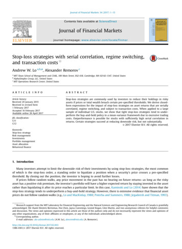
A.W. Lo, A. Remorov / Journal of Financial Markets 34 (2017) 1–157Fig. 2. Two-Week Stop-Loss Strategy Performance for AR(1) Process. Performance statistics for stop-loss strategy with I J 10 , start level of 0%, andvarying stop levels. All statistics are measured relative to the buy-and-hold, so that the value for the buy-and-hold strategy is subtracted from that of thestop-loss strategy.there is improvement in the left tail. In contrast, the two-week strategy yields higher skewness in almost all situationsbecause the effect on the right tail is quite marginal, whereas the downside risk is cut, especially if serial correlation is high.The one-day strategy improves maximum drawdown only in cases of positive serial correlation; the two-week strategydoes so for quite a few values of negative correlation as well. This difference is due to the fact that while the one-day strategycuts downside risk, it also incurs high transaction costs and produces poor returns when serial correlation is negative.In conclusion, the returns and CE of stop-loss strategies depend heavily on serial correlation and volatility, outperformingthe buy-and-hold strategy only for high values of these parameters. For an investor with preferences for positive skewnessand a lower drawdown, the two-week strategy is quite attractive since it is able to reduce downside risk consistentlywithout incurring too much in trading costs while maintaining most of the upside potential.4.2. Regime-switching processWe now consider a Markov regime-switching (MRS) process for daily returns:rt μit σit ϵt , ϵt WN (0, 1),(14)where it {1, 2} is the regime indicator that evolves according to a discrete Markov chain with transition probabilitymatrix P: p11 p12 P , p21 p22 (15)so that pij (it 1 j it i ). In the “bull market” regime, the risky asset's returns are distributed as N (μ1,“bear market” regime, its returns are distributed as N( μ , σ ), where μ2222 21 ),σand in theμ1.There are three sets of parameters: the means, μ1, μ2 , the volatilities, σ1, σ2, and the transition probability matrix, P. Wevary each of them to see how the stop-loss and buy-and-hold strategies perform relative to each other. Table 1 lists theparameter values considered, which were chosen to capture a representative range of empirical characteristics for U.S.equities. The more extreme negative values of μ2 and σ2 represent stock-market crashes. Both transition probability matrices we consider imply that these negative regimes are not rare but occur much less frequently than the positive regimes(20% and 14% of the time for P1 and P2, respectively). For each unique set of parameter values, we run 100,000 simulationsover a 252-day horizon; standard errors are provided in the Appendix.Figs. 3 and 4 show the performance statistics for the one-day and two-week stop-loss strategies relative to the buy-andhold strategy. The stop-loss strategy produces lower returns in almost all cases; it is able to outperform in terms of CE when

8A.W. Lo, A. Remorov / Journal of Financial Markets 34 (2017) 1–15Table 1Parameter Values of MRS Process Simulations. Table 1 lists the parameter values of the simulationsfor the MRS process. The means, μ1, μ2 , and standard deviations, σ1, σ2 , are annualized. The highervalues ofσ2 and the more extreme low values of μ2 capture stock market crashes. There are twocases for the transition probability matrix P : P1, when there is little switching out of regimes, andP2, when there is frequent switching.Parameters(μ1,Values Consideredμ2 )σ1σ2(10%, 10%) , (15%, 20%) , (20%, 30%)PP1 20% , 30%40% , 80% 0.990.040.01 0.96,P 0.96 2 0.250.04 0.75 volatility is high in the bear regime. Performance is better when the expected return in the bear regime is low and whenthere is little switching between regimes. The intuition behind this is that for the stop-loss strategy to outperform, it mustswitch out of the risky asset during negative regimes. Further, the negative regime should last for a considerable amount oftime so that the relative gain of investing in the risk-free asset will offset transaction costs.The improvement in CE in situations of high volatility in the bear regime happens for two reasons. First, when volatility isvery high, the stop-loss strategy is more likely to be triggered, correctly divesting when expected returns are negative.Second, the high volatility in the negative regime results in a low CE for a mean-variance investor, so the risk reduction dueto holding the risk-free asset produces significant benefits relative to the buy-and-hold strategy.When it comes to skewness and kurtosis, the results are similar to those of the AR(1) process. The one-day strategy giveslower skewness, while the two-week strategy gives higher skewness in comparison to the buy-and-hold strategy. Furthermore, while the one-day strategy improves maximum drawdown over the buy-and-hold strategy in about half the cases(again, for high volatility in the bear regime), the two-week strategy does so in all situations

sample of individual U.S. stocks, we show that tight stop-loss strategies tend to under-perform the buy-and-hold policy in a mean-variance framework due to excessive trading costs. Outperformance is possible for stocks with sufficiently high serial correlation in returns. Certain strategies succeed at reducing downside risk, but not substantially.