Transcription
Appl. Math. Inf. Sci. 9, No. 1, 473 -483 (2015)473Applied Mathematics & Information SciencesAn International tivity Analysis of Inefficient Supply ChainsM. Sanei, Sh. Banihashemi and F. SouraniDepartment of Applied Mathematics, Islamic Azad University, Central Tehran Branch, Tehran, IranReceived: 30 Jun. 2013 , Revised: 16 Dec. 2013, Accepted: 20 Dec. 2013Published online: 1 Jan. 2015Abstract: The present study is an attempt toward improving the performance of members of supply chain. Improvement of two-stagesupply chains is three cases. Inefficients suppliers are improved or inefficient manufactures are improved or both of them are improved.First, New sub-perfect supply chain production possibility set is obtained with efficiency score of α for inefficient suppliers and onlyall DEA inefficient suppliers are improved. It is proved that as the efficiency score of all points on the main frontier supposed tobe 1, the efficiency score on the new frontier is α .Second the procedure is applied for those supply chains which are inefficient inmanufacture performance and only all DEA inefficient manufacturers are improved and the last one, it is used to improve the supplychains which are inefficient in supplier and manufacture performances at the same time. In the last two ones it is shown that thereare improvements in inefficient manufactures or in both of them at the same time but the improved efficiency is not able to appraiseexactly. Overall performance score has an improvement in all cases and the supply chain management can choose the best strategies tomaximize overall efficiency score. This paper develops procedures which are referred to each case for performing a sensitivity analysisof the inefficient supply chains in constant returns to scale (CRS). The real case is applied to accept this approach.Keywords: Data Envelopment Analysis (DEA), Supply Chain Management (SCM), Sensitivity Analysis, Supply Chain, Efficiency1 IntroductionA supply chain is the combination of equipment,suppliers, manufactures, distributors, retailers and methodof controlling inventory, purchasing and distribution, thatit tends to improve the way your company finds rawmaterials it needs to produce a product or service and todeliver it to customers, for example, China ConstructionBank [1, 2]Supply chain effective management has been widelyaccepted as an important means for supplier ormanufacturer or distributor, to obtain the best andhigh-quality products and services by the least cost andthe most profit. The evaluation of the performance andimprovement are a great importance and necessity forrecognizing in supply chain management (SCM). Insupply chain management (SCM), although decreasingthe cost and increasing profit is very important, but alsopartnerships with together is a significant factor forenhancing competitiveness. Among many evaluationmethods, data envelopment analysis (DEA) is one of thebest ways for assessing the relative efficiency a group ofhomogenous decision making units (DMUs) that usemultiple inputs to produce multiple outputs, originatedfrom the work by Charnes et al [3]. DEA has been applied Correspondingto evaluate the supply chain performance in several workssuch as, [4–8] and so on. The traditional DEA modelscan’t be applied directly to the supply chain case becauseclassical DEA treats each DMU, supply chain, as a blackbox and for example in a supplier-manufacture chainconsiders only the initial inputs from suppliers and finaloutputs at the very end of downstream members in theperformance evaluation. For the complex nature of supplychain, those intermediate products or linking activities areignored. Then, several authors have attempted to accountthese links and consider supply chain as a network DEAby multi-stage [9]. The network DEA modelproposed [10] has a multi-stage structure as an extensionof the two stage supply chain [11] and DEA modelproposed in [12]. In recent years, one of the mostimportant issues in DEA is the sensitivity analysis ofefficient DMUs. In 1985, sensitivity analysis of CCRmodel for a specific efficient DMU with a single outputwas initiated by Charnes et al. [13]. In 1990 Charnes andNeralic considered additive model and they obtainedsufficient conditions for remaining efficient [14]. Then in1992, Charnes et al. obtained a specific stability region byusing L1 and L [15]. These researchers have studied themethods which simultaneous proportional change isauthor e-mail: shbanihashemi@atu.ac.irc 2015 NSPNatural Sciences Publishing Cor.
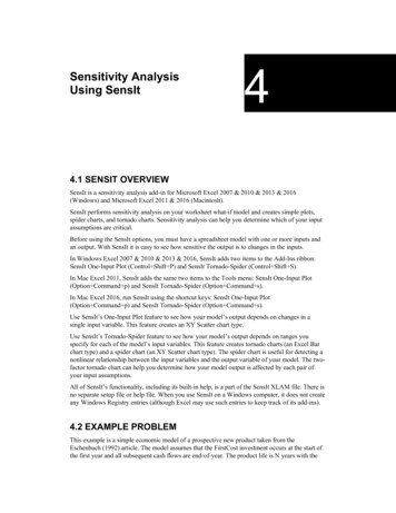
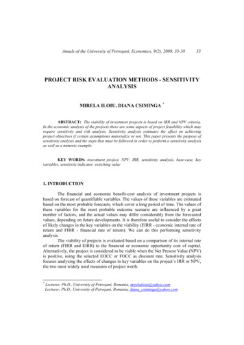
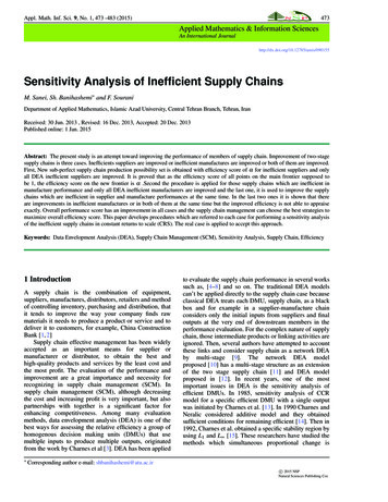
474assumed in inputs and outputs for a specific efficientDMU under evaluations. Then Zhu (1996) provides amodified DEA model to compute a stability region whichDMU under evaluation remains efficient [16].In 1998 Seiford and Zhu developed a procedure todetermine an input stability region (ISR) and an outputstability region (OSR) for efficient DMU [17]. Theystated that an efficient DMU will remain efficient after theinput increases or output decreases if and only if suchchanges occur with in the ISR or OSR [17], and thissubject are considering in recent years. Jahanshahloo etal. [18] extended the largest stability region for BCCmodelandAdditivemodelbysupportinghyperplanes [19] for DMU under evaluation which allinputs and outputs of DMUs except DMU underevaluation are assumed fixed. In some works sensitivityanalysis is based on the super efficiency DEA approach inwhich the efficient DMU under evaluation is not includedin the reference set [20, 21, 23]. Sensitivity analysis of aninefficient DMU is studied less than sensitivity of anefficient DMU.In 1992, Charnes, Haag et al. obtained animprovement for inefficient DMU by using Chebychevnorm [15]. The model dealt with improvements in bothinputs and outputs that could occur for an inefficientDMU before its statues would change to efficient.In the recent years sensitivity analysis of inefficientunits has been more studied. In 2011 Jahanshahloo et al.supposed that DMU under evaluation is inefficient by theefficiency score of θo and θo α 1 which α is a fixedconstant and defined by the manager .They obtained thenew frontier Tv′ with efficiency score of α . They provedthat as the efficiency score of all points on the mainfrontier supposed to be 1, the efficiency score on the newfrontier is α [20].But sensitivity analysis of supply chain is still inabsence. Improvement in supply chain performance isone of the most important mentioned advantages ofprogress supply chain.In 2011, Yang et al. [11] defined two types of supplychain production possibility sets ,which are proved to beequivalent to each other and based upon the productionpossibility set, a supply chain CRS DEA model isadvanced to appraise the overall technical efficiency ofsupply chain and they obtained the benchmarking unitsfor inefficient supply chains.Inefficiency of two-stage supply chains is in threecases. Supplier is inefficient or manufacture is inefficientor both of them are inefficient. This paper developsprocedures for performing a sensitivity analysis of theinefficient supply chains in three cases. We consider twostage supply chain which includes supplier andmanufacture and the supply chain is under the control of aunique decision maker. By using [11] and the proposedmethod, new sub-perfect supply chain productionpossibility set is obtained with efficiency score of α forinefficient suppliers and in this case it has been focusedmainly around that only DEA inefficient suppliers havean improvement. It is proved that as the efficiency scorec 2015 NSPNatural Sciences Publishing Cor.M. Sanei et. al. : Sensitivity analysis of inefficient supply chainsFig. 1: A supplier-manufacturer chainof all points on the main frontier supposed to be 1, theefficiency score on the new frontier is α . By differentways such as decreasing inputs, increasing outputs orcombination strategies, DEA inefficient suppliers with can obtain efficiency score of αefficiency scores of θsoand also the decision maker can choose the bestimprovement strategies to maximize the overallperformance score. Next the model is applied for thosesupply chains which are DEA inefficient in manufactureperformance and only all DEA inefficient manufacturersare improved .The last one , it is used to improve thesupply chains which are inefficient in supplier andmanufacture performance at the same time.In these caseswe show that there are improvements in inefficientmanufactures or in both of them at the same time but theimproved efficiency is not able to appraise exactly and wehave improvement in overall performance score too. Whatwe do is that the inefficient supply chains are appraisedrespected to a new frontier with efficiency score which isa fixed number (and defined by the manager). Thedecision maker gives a chance or fortune to them untilthey can have an improvement and finally the overallefficiency score of supply chain is improved and theoverall performance of supply chain is progressed and itis contented the decision maker.This paper proceeds as follows. The next sectionrepresents some basic DEA models. Section 3 develops aproposed method for improving the overall performanceof inefficient supply chains. Section 4 is a real worldapplication and the proposed method is applied toevaluate the performance of banking chains in a bigChinese commercial bank. Finally conclusions are givenin section 5.2 BackgroundSuppose there are N two-stage supplier-manufacturerchains as shown in Fig. 1. where S and M representsupplier and manufacturer, respectively. The variable X isthe input vector of the supplier (S) and the variable Z isthe output vector of the supplier and is also an input ofmanufacturer (M). The variable Y is the manufacturer’soutput vector.Any supplier consumes P inputs to generateK intermediate products, and the manufacturer consumesthose intermediate products to produce Q outputs.Specially for the j th SC, the inputs and outputs for thesupplier are X p j (p 1, 2, ., P) and Zk j (k 1, 2, ., K) ,and they are Zk j (k 1, 2, ., K) and Yq j (q 1, 2, ., Q)for manufacturer, respectively.
Appl. Math. Inf. Sci. 9, No. 1, 473 -483 (2015) / www.naturalspublishing.com/Journals.aspDefinition 1(Perfect supply chain CRS productionpossibility set [11]). (x p , yq ) Nj 1 λ jS x p j x p , p 1, 2, ., P Nj 1 λ jS zk j zk , k 1, 2, ., K NMTSC P j 1 λ j zk j zk , k 1, 2, ., K Nj 1 λ jM yq j yq , q 1, 2, ., Q j 1, 2, ., Nλ jS , λ jM 0,(1)Definition 2(Sub-perfect supply chain CRS productionpossibility set [11]). (x p , yq ) Nj 1 λ j x p j θS j x p , p 1, 2, ., P k 1, 2, ., K Nj 1 λ j zk j zk , Nk 1, 2, ., KTSC SP j 1 λ j zk j zk , Nj 1 λ jM yq j /θM j yq , q 1, 2, ., Q λ jS , λ jM 0,j 1, 2, ., N(2)Theorem 1.TSC P TSC SPConsider DMU j , ( j 1, ., n ), where each DMUconsumes m inputs to produce s outputs. Suppose that theobserved input and output vectors of DMU j areX j (x1 j , ., xm j ) and Y j (y1 j , ., ys j ) respectively, andlet X j 0 and X j 6 0 and Y j 0 and Y j 6 0.The production possibility set Tc and Tv are defined asfollows:)(nnTV (X,Y ) X ((X,Y ) X j 1j 1nnnj 1j 1) λ X j ,Y λ jY j , λ j 1, λ j 0, j 1, ., njj 1 ′′′Proof.See [20]Attention 1. There is one- to- one correspondencebetween E and E ′ .Attention 2. There is one-to-one correspondence betweenTv and Tv′ frontier points.Proof.See [20]Theorem 3.The efficiency score of each point on the Tv′frontier is α in Tv .Proof.See [20]jAnd the new production possibility set Tv′ :(Theorem 2.The efficiency score of each point of E ′ in Tv isα. λ X j ,Y λ jY j , λ j 0, j 1, ., nLet the set of extreme efficient DMUs in Tv be E. Bydetermining the set of E, the set of E ′ is defined asfollows [20]: 1′′ ′′ ′X j ,Y j , j EE X j ,Y j X j ,Y j αTv′In the recent years data analysis of inefficient units hasbeen more studied. In 2011 Jahanshahloo et al. supposedthat DMU under evaluation is inefficient by the efficiencyscore of θo and θo α 1 which α is a fixed constantand defined by the manager .They obtained the newfrontier Tv′ with efficiency score of α . They proved thatas the efficiency score of all points on the main frontiersupposed to be 1, the efficiency score on the new frontieris α .Then by using different ways such as decreasinginputs, increasing outputs or combination strategies,DMUo with efficiency score of θo can obtain efficiencyscore of α and has an improvement for α θo inefficiency.[20]Proof.See [20]Proof.See [11]Tc 475(X ,Y ) X 1α λ j X j ,Yj E′ λ jY j , λ j 1, λ j 0, j Ej Ej E)To find extreme efficient DMU in BCC model, Andersonand Petersen (AP) model is solved for each DMU [24]:AP : min θoS.t. nλ x θo xio , i 1, 2, ., mj 1 j ijj 6 o nj 1 λ j yr j yro ,r 1, 2, ., sj 6 o nj 1 λ j 1j 6 oλ j 0, j 1, ., n, j 6 0(3)3 Proposed methodSuppose there are N two-stage supplier-manufacturerchains as shown in Fig. 1. where stage S represents thesupplier and the stage M represents a manufacturer,respectively.Any supplier consumes P inputs to generateK intermediate products, and the manufacturer consumesthose intermediate products to produce Q outputs. Theinputs and outputs for the j th supplier areX p j (p 1, 2, ., P) and Zk j (k 1, 2, ., K) , and they areZk j (k 1, 2, ., K) and Yq j (q 1, 2, ., Q) for the j thmanufacturer, respectively.Consider N same supply chains called DecisionMaking Units (DMUs) in DEA literatures, denoted byDMU1 , DMU2 , ., DMUN in the context. In most practicalsituations of supply chain management, the chainoperated under the fulfillment of demand fromconsumers.The performance of a supply chain (SC) isattributed to two main factors: the performances of all SCmembers, and the co-operation of its members. It meansthat the performance of each supply chain’s member isvery important and it is influenced on the overall supplychain efficiency. The influence of supply chain thought onorganizational strategy has also significant reflecting. Asindependent decision makers, each supply chain membersc 2015 NSPNatural Sciences Publishing Cor.
476M. Sanei et. al. : Sensitivity analysis of inefficient supply chainsmaximized its own technical efficiency, thus eliminatesthat of other members and even of the overall chain.Suppose that the evaluated supply chain is DEAinefficientwiththetechnicalefficiencyθo 1 (o 1, 2, ., N) . The supply chain is under thecontrol of a unique decision maker.The goal is to improvethe inefficient supply chain to achieve some desired levelof performance which is defined by the supply chainmanagement. This overall inefficiency of supply chainhappens when supplier or manufacturer is inefficient orboth of them are inefficient at the same time.Thereforethese inefficiencies are considered in three cases. Theproposed method is employed to improve just inefficientmember of supply chain and it is deemed the overallchain and also the other members of SCs.The inefficientsupply chains are appraised respected to a new frontierwith efficiency score which is a fixed number (anddefined by the manager). The decision maker gives achance or fortune to them until they can have animprovement.In case 1 the exact value of efficiency isobtained and overall performance of supply chain isimproved too. In case 2 and 3 it is shown that there areimprovements in manufacturer and both of them at thesame time and overall performance score of supply chainhas an improvment too but the exact score or value is notappraisable.Case1. Suppose that the evaluated supply chain is DEAinefficient. In the first case, it has been focused mainlyaround that only DEA inefficient suppliers have animprovement. They are evaluated by Constant Returns toScale (CRS) assumption. The new sub-perfect frontierwith efficiency score α ( α is a fixed constant which isdefined by the supply chain manager) is obtained and theDEA inefficient suppliers are evaluated by the newfrontier. Denote the production possibility set for allsupply chains by [11]:be rewritten as the following programming: (X,Y ) Nj 1 λ j θs j X j X, Nj 1 λ j Z j Z, NTSC SP j 1 λ j Z j Z Y Y Nj 1 λ j ϕM j j λ j 0, j 1, 2, ., N(4)By the above Production Possibility Set (PPS) θd the dthsupply chain’s DEA efficiency score obtained by thefollowing LP problem:θd min θ Nj 1 λ j X j θ Xd , Nj 1 λ jY j Yd ,(X j ,Y j ) TSC SPλ j 0, j 1, 2, ., N(6)We know that the Production Possibility Set of supplier isas follows:TCS (N(X, Z) λ jS X jN X,j 1λ jS Z j Z,λ jS 0, jj 1)(AP) model is employed to find all extreme efficientsuppliers. Let the set of extreme efficient suppliers in TCS′be ECS . Having determined ECS , ECSis defined asfollows:′ECS X j′ ,Z ′j X j′ ,Z ′j 1X j , Z j , j ECS .α′ isThe new production possibility set for suppliers TCSintroduced by:′TCS ((X ′ , Z ′ ) α1 λ jS X j ′ X ,j ECSλ jS Z j′ Z ,λ jS 0, j ECSj ECS)Supposed that supplychaind is inefficient and it is andinefficient in supplierd by the efficiency score of θsd α 1 which α is a fixed constant and defined byθsd′ with efficiency score ofthe manager. The new frontier TCSα is obtained. We know that as the efficiency score of allpoints on the main frontier supposed to be 1, theefficiency score on the new frontier is α . The CCR modelof the d th (d 1, 2, ., N) supplier (the supplier in thed th′ is computed by the following model:SC) in TCSθs′ min θss.t. Nj 1 λ jS x′p j θs x′pd , p 1, 2, ., P Nj 1 λ jS z′k j z′kd , k 1, 2, ., Kλ jS 0,j 1, 2, ., N(5)(X , Z ,Y ) are points that located at the frontierconstructed by the sub-perfect supply chain CRSProduction Possibility Set. Also ESC SP is considered asall extreme efficient supply chains. The above model canc 2015 NSPNatural Sciences Publishing Cor.θd min θs.t. Nj 1 λ j X j θ Xd Nj 1 λ jY j Yd Nj 1 λ j X j θs j X j Nj 1 λ j Z j Z j Nj 1 λ j Z j Z j Y Nj 1 λ jY j ϕMjjλ j , λ j 0, j 1, ., N(7)For improving inefficient supply chains and to find thenew supply chain frontier, first of all the extreme pointsofTSC SP should be found. These points are called thesetESC SP . They are sub set of extreme points of TCS . In′the sequel, the set ESC SPis found and defines as follows:′ESC SP ′′′′′{(X j , Z j ,Y j ) X j , Z j ,Y j ′
Appl. Math. Inf. Sci. 9, No. 1, 473 -483 (2015) / www.naturalspublishing.com/Journals.asp Y }. Then T ′θs ′ j X j′ , Z j , ϕMj jSC SP is as follows:′TSC SP ′ (X ′ ,Y ′ ) α1 λ j X j θs ′ j X , j ESC SP ′ λZ Z, jj j ESC SP ′λZ Z, j j j ESC SP ′ λ jY j ϕM j Y , j ESC SP 0,j Eλ jSC SP (8) ,Y be anProof.Let M ′ with coordinate XM ′ , ZM′M′′arbitrary extreme efficient point in ESC SP. By definition, we have (XM , ZM,YM ) ESC SP .At the first step, we are going to prove M ′ is efficient in′′TSC SP . By contradiction, let M ′ not be efficient in TSC SP.According to the assumption:( ′X j α1 X j ′Y j Y j and we have:min θM′s.t. j E ′ are the CCR efficiency score of theWhere θs ′ j and ϕMjsupplier and manufacturer in the jth supply chainrespectively.Then by using [11] sub-perfect supply chain CCRproduction possibility set is obtained and modeled asfollows:θd ′ min θ′s.t. j E ′λ j X j θ Xd′ ′SC SP′′λ jY j Yd′ ′ j ESC SP′λ j 0, j ESC SP′′ ′(X j ,Y j ) TSC SP(9)The above model can be rewritten as the followingprogramming:θd ′ min θ′s.t. j E ′λ j X j θ x′ ′SC SPd′′λ j y j y′d ′ j ESC SP′′λ j X j′ θs ′ j Xd ′ , j ESC SP′′λ j Z j Zd ′ , j ESC SP′′λ j Z j Zd ′ , j ESC SP Y ′ ,′λ jY j ϕM j ESC SPjd′′λ j , λ j 0, j ESC SP477(10)By this procedure, new sub-perfect supply chain′production possibility set frontier which is called TSC SPis obtained for inefficient supply chains which areinefficient in suppliers and only DEA inefficient suppliershave an improvement. It is proved that as the efficiencyscore of all points on the main frontier supposed to be 1,the efficiency score on the new frontier is α . By differentways such as decreasing inputs, increasing outputs orcombination strategies, DEA inefficient suppliers with can reach to the new frontierefficiency scores of θso′TSC SP and also the decision maker can choose the bestimprovement strategies to maximize the overallperformance score .Now by following theorems and′lemma, It is shown that every point on TSC SPfrontier hasan efficiency score α .′Lemma 1.M ′ ESC SPif and only if M ′ is an extreme′efficient unit in TSC SP.′λ j X j θM′ XM′ θM′′′λ jY j YM′ YM , j ESC SP′′′(X j ,Y j ) TSC SP′λ j o, j ESC SPSC SP1α XM Suppose that the optimalsolution of above mentioned problem is λ , θM ′ . By contradiction suppose θM ′ 1. So we get ′′λ j X j θM ′ XM′ j ESC SP ′ ′λ j Y j YM′ YM , j ESC SP′′′ (X ,Y ) TSC SP j j′λ j o, j ESC SPBy multiplying the first constraint to α , we get ′′λ j (α X j ) θM ′ (α XM′ ) j ESC SP ′ ′λ j Y j YM′ YM , j ESC SP (X ′ ,Y ′ ) T ′ SC SP j j′λ j o, j ESC SP′According to definition ESC SP and ESC SP: j ESC SP λ j X j θM ′ XM j ESC SP λ j Y j YM , ′ (X j ,Y j ) TSC SP λ j o, j ESC SP The last one has a feasible solution λ , θM ′ 1 for thecorresponding problem of M ESC SP that iscontradiction with M ESC SP .′So M ′ is efficient in TSC SP. At the sequel it is going′′to prove that M is an extreme unit in TSC SP. In′contradiction, suppose that M to be a non-extreme′efficient unit in TSC SP. Let the set of extreme points in′TSC SP be:n ′ ′ ′ ′ ′ ′ oX1 , Z1 ,Y1 . Xt , Zt ,Yt .It has; ,Y XM ′ , ZM′M′t λjj 1 ′ ′ ′ X j , Z j ,Y j ,t λ j 1, λ j 0,j 1, .,tj 1c 2015 NSPNatural Sciences Publishing Cor.
478M. Sanei et. al. : Sensitivity analysis of inefficient supply chainsorThen: (XM′ , ZM ′ ,YM ′ ) ( 1 X , Z ,Yα M M Mt λjj 1 1 X j , Z j ,Y j ,αtj 11 X , Z ,Yα M M M ttj 1j 11 (α λ jY j ) , λ j 1,XM t λ j X j , ZM j 1t λ j 1,t λ j X j ,j 1t λ j Z j ,λ j 0,tj 1, .,tYM j 1t λ jY j j 1λ j 0, j 1, .,t .j 1therefore:ttj 1tj 1 (XM , ZM,YM ) ( λ j X j , λ j Z j , λ jY j )t λjj 1 X j , Z j ,Y j ,j 1t λ j 1,j 1λ j 0, j 1, .,t ,Y ) as aIt is represented M with coordinates (XM , ZMMconvex combination of extreme efficient points in TSC SPand this is in contradiction with the assumption. Hence,′′M ′ ESC SPis an extreme efficient unit in TSC SP. ,Y Conversely if M ′ with coordinates XM ′ , ZMbean′M′′arbitrary extreme efficientpointinT,itisclaimedSC SP that α XM′ , ZM′ ,YM′ is an extreme efficient point in ,Y not be inTSC SP . By contradiction, let α XM ′ , ZM′′MESC SP . So we have: (α XM′ , ZM ′ ,YM ′ ) j ESC SP λ j 1 , λ j 0, j ESC SP .j ESC SPc 2015 NSPNatural Sciences Publishing Cor. ′λ j Z j ,′j ESC SP′j ESC SP′λ jY j )′j ESC SPλ j 1 λ j 0, j ESC SP . ,Y Then XM ′ , ZMis represented as a convex′M′′combination of extreme efficient points in TSC SP. It is incontradiction with our assumption.So the prove is ,Y E ′completed and XM ′ , ZM′SC SP .M′Theorem 4.There is a one-to-one correspondence′between TSC SP , TSC SPfrontier points. ′ ′ Proof.Let M ′ with coordinate XM′ ′ , ZMbe an′ ,YM ′′arbitrary point on the TSC SP frontier. Each point on the′TSC SPfrontier is extreme efficient or a non-extremeefficient point.As we know the set of extreme efficientsupply chains in TSC SP is ESC SP and the set of extreme′′efficient supply chains in TSC SPis ESC SP. ′ 1.if M with coordinate XM′ , ZM′ ,YM′ be an arbitrary′extreme efficient point on TSC SPBy lemma. 1′′M ESC SP .There is a one- to-one correspondence′′between ESC SP and ESC SP. Because the set ESC SPis generated from ESC SP . So there is a one- to-onecorrespondence between extreme points on TSC SP′and TSC SP.′2.if M be an arbitrary non- extreme efficient point on the′frontier, it is shown that there is a one-to-oneTSC SPcorrespondence between non-extreme efficient points′on the TSC SP and TSC SP.There are t extreme efficient′points on TSC SP so that: (XM ′ , ZM′ ,YM ′ ) t µjj 1t ′ ′ ′ X j , Z j ,Y j , µ j 1, µ j 0,j 1, .,tj 1Then: (XM ′ , ZM′ ,YM ′ ) (1αtttj 1j 1j 1 µ j X j , µ j Z j , µ jY j ), µ j 1, λ j X j , Z j ,Y j , ′λ j (X j ),tµ j 0, j 1, .,t.j 1λ j 1λ j 0, j ESC SP .j ESC SP λ j X j ,λ j Z j ,λ jY j ),(α XM′ , ZM ′ ,YM ′ ) (j ESC SPj ESC SPj ESC SP ′j ESC SPj 1 λ j Z j ,λ j 1, λ j 0, j ESC SP .j ESC SP (XM′ , ZM ′ ,YM ′ ) ( λ j 1, λ j 0, j 1, .,t. 1λ j ( X j ), λ j Z j , λ jY j ),αj ESC SPj ESC SPj ESC SP ttj 1j 1 (XM , ZM,YM ) ( µ j X j , µ j Z j ,t µ j 1,j 1t µ jY j ),j 1µ j 0, j 1, .,t.
Appl. Math. Inf. Sci. 9, No. 1, 473 -483 (2015) / www.naturalspublishing.com/Journals.aspWe prove that M to be on the TSC SP frontier. Assumecontradiction that M is not on frontier .it is evaluatedby the following model:min θMs.t. j ESC SP λ j X j θM XM j ESC SP λ jY j YM(X j ,Y j ) TSC SPλ j 0, j ESC SP(11)(λ , θM )is the optimal solution for theAssume thatprevious problem. Respecting to contradictionassumption, it can be obviously seen that θM 1 .Then, the first constraint is multiplied to α1 , so: ′λJ X j θM XM′ ′ j ESC SP ′ λ j Y j YM′ YM j E ′ SC SP′ ′ (X j ,Y j ) TSC SP′λ j 0, j ESC SPThe above model has a feasible solution (λ , θM 1 )′and this is in contradiction with M ′for M ′ TSC SP′that is a non-extreme efficient unit on the TSC SPfrontier and it is completed our proof.Theorem 5.The efficiency score of each point on the′TSC SPfrontier is α in TSC SP . ′ ,Y ′ Proof.Let M ′ with coordinate XM′ ′ , ZMbe an′M′′arbitrary point on the TSC SPfrontier. Each point on the′TSC SPfrontier is extreme efficient or a non-extremeefficient point. The following model is employed toevaluate the point M ′ in TSC SP :min θM′s.t. j ESC SP λ j X j θM′ ( α1 XM ) j ESC SP λ jY j YM′ YM(X j ,Y j ) TSC SPλ j 0, j ESC SP(12)479A feasible solution for this model is: θM (1 ε) 1, λM 1, λ j 0, ( j Esc sp, j 6 M)αIt means that DMUM is inefficient and this is incontradiction with the assumption. Hence θM ′ α and itis completed the proof.Case 2. Suppose that the evaluated supply chain is DEAinefficient. In the second case, it has been focused mainlyaround that only inefficient manufacturers have animprovement. In this case we cannot use the sub-perfectCRS DEA model. Because the sub-perfect CRS DEAmodel deem the input changes of manufacturers oreffective of intermediate units.It means that thesub-perfect CRS DEA model evaluated the changes of theoverall input vector and overall output vector of supplychain and it does not consider the changes of intermediateunites. In this model we have one input vector formanufacturer that it is output vector for supplier. But wewant to change just the input vector of manufacturer. Sowe should have two input vectors for manufacturer thatone of them is the output vector for supplier and the otheris new input vector that is injected to manufacturer andthey are called Z1 and Z2 respectively. The case is shownin Figure 2.Fig. 2: There are two input vectors for manufacturer.On the other hand, we know supply chaino is inefficientand it is inefficient in manufactureo. By (1) the ProductionPossibility Set (PPS) is obtained and θMC Sp is gained bythe following LP problem.min θMC SPNThemodelhasafeasiblesolution(θM′ α , λM 1, λ j 0, ( j ESC SP , j 6 M))Hence the optimal θM′ , denoted by θM ′ , is not greaterthan α . It will be representedθM ′ α . In contradiction, assume that θM′ α .Therefore θM ′ α ε for someε 0. By applying Model (12): 1α ε λ j X j θM′ XM′ θM′ α XM α XMj ESC SP ε 1 Xα M λ jY j YM′ YMj ESC SP(X j ,Y j ) TSC SPλ j 0, j ESC SPs.t. λ jS X j θMC SP Xoj 1N λ jS Z1 j Z1oj 1N(13) λ jM Z2 j Z2oj 1N λ jMY j Yoj 0λ jS 0,λ jM 0,j 1, 2, . . . , N(AP)model is employed to find all extreme efficientsupply chains [24]. Let the set of extreme efficient supplychains in TMC Sp be EMC SP . Having determinedc 2015 NSPNatural Sciences Publishing Cor.
480M. Sanei et. al. : Sensitivity analysis of inefficient supply chains′EMC SP , EMC SPis defined as follows:′EMC SP X j′ , Z1′ j , Z2′ j ,Y j′ X j′ , Z1′ j , Z2′ j ,Y j′ 1 X j , Z1 j , Z2 j ,Y j , j EMC SPβ′We introduce the new production possibility set TMC SP: ′ ′ (X ,Y ) j EMC SP λ jS X j X ′ , j EMC SP λ jS Z1 j Z ′ , 1′M Z 1Z ′ ,λTMC SP j EMC SP j 2 jβ j EMC SP λ jMY j 2Y ′ , λ S , λ M o, j E MC SPjj′isBy the above new Production Possibility Set, θMC SPobtained by the following LP problem:′min θMC SPNs.t.′Xo λ jS X j θMC SPj 1N λ jS Z1 j Z1oj 1N λ jM Z2 jj 1N(14)1 Z2oβ λ jMY j Yoj 1λ jS 0,λ jM 0,j 1, . . . , NLike the case 1, there is the new frontier but the efficiencyscore on it does not exactly determined. What we sure arethat the frontier is close to the main frontier and thedecision maker gives chance to those inefficientmanufactures to improve themselves. They are DEAinefficient and they cannot obtain efficiency score 1 butthey can gain the constant which is closer to 1 and definedby the manager and satisfy him.They have absolutely animprovement but the value of the improvement is notexactly determined. What we do is that the inefficientsupply chains which are inefficient in manufacturersperformance are appraised respected to a new frontierwith efficiency score which is a fixed number (anddefined by the manager). SCo is DEA inefficient and it isinefficient
evaluation are assumed fixed. In some works sensitivity analysis is based on the super efficiency DEA approach in which the efficient DMU under evaluation is not included in the reference set [20,21,23]. Sensitivity analysis of an inefficient DMU is studied less than sensitivity of an efficient DMU.In 1992, Charnes, Haag et al. obtained an