WIXLIB

Sensitivity Analysis of SWAT Using SENSANZhulu LinDepartment of Crop and Soil SciencesThe University of Georgia, Athens, GA 30602linzhulu@uga.eduModel sensitivity analysis can help us assess the relative sensitivity of model output withrespect to the changing of model parameters. It often is the first step in a modelcalibration exercise whereby key model parameters can be identified. This note brieflyillustrates how to utilize SENSAN (a PEST companion program) and MS Excel toconduct sensitivity analysis for the SWAT model. SENSAN adopts a local sensitivityanalysis method which takes a one-at-a-time (OAT) approach. In this approach, theimpact of changing values of each model parameter on the model outputs is evaluatedone at a time. That is, model output responses are determined by sequentially varyingeach of the model parameters and by fixing all other parameters to their nominal values.Often these nominal values are taken from literature. The combination of nominal valuesfor all the model parameters under inspection is called the “control” scenario. While thelow computational cost is one of the main advantages of the OAT approach, the OATmethod has many limitations when applied to complex (nonlinear) environmental modelssuch as SWAT. One limitation of the OAT methods is that they do not account for anyinteraction between model parameters (if any exists) since the sensitivity analysis isperformed for one parameter at a time by fixing all other parameter at constant nominalvalues. Furthermore, in a local method, parameters are changed over small intervalsaround their nominal values. These nominal values represent a specific point of theparameter space (i.e., the “control” scenario). Results of such a local method are thusdependent on the choice of this point, and the model behavior is identified only locally inthe parameter space (namely, around the selected point). The farther the perturbation inparameter moves away from the nominal value, the less reliable the analysis results willbe. It is acceptable only if the input-output relationship can be adequately approximatedthrough a first-order polynomial (i.e., linear input-output relationship). However, if themodel shows strong nonlinearity (like many hydrologic and water quality models)between model parameters and model outputs then a change in the selected nominalvalues (“control” scenario) will provide totally different sensitivity results. Therefore,care should be exercised when interpreting the sensitivity analysis results from theSENSAN program.1

1. SENSAN Files1.1 SENSAN control fileLike the PEST program, SENSAN’s master file is the SENSAN control file with a fileextension name .sns (see Example 1). A SENSAN control file must begin with scf asits first line (Line 1). The remaining SENSAN control file consists of 4 blocks; eachblock begins with a narrative line. As in the PEST control file, each narrative lineconsists of an asterisk followed by a space and the block name. The block names have tobe the same as those shown in Example 1. They are “control data”, “sensanfiles”, “model command line”, and “model input/output”. In block“control data”, don’t worry about noverbose (Line 3). In Line 4, the firstnumber (10) is the total number of model parameters, with respect to which, thesensitivity of the model’s outputs will be analyzed; while the second number (5) is thetotal number of model outputs. In Line 5, the first entity (1) is the number of templateand input file pairs; while the second entity (1) is the number of instruction and outputfile pairs. The two ones (1’s) correspond to Lines 14 and 15, respectively. Since we usethe SWAT linkage interface developed by Jing Yang in the Swiss Federal Institute forEnvironmental Science and Technology (see “Running SWAT in A Breeze” for detailson how to use the linkage interface) to run SWAT, only one pair of template and modelinput files is needed. All the model output variables (such as surface runoff, total wateryield, sediment yield, and phosphorus loads) are read from the output.std file in thisexample, so only one pair of instruction and model output files is needed, as well. Don’tworry about the entities in C3 and C4 in Line 5.Ln123456789101112131415C1C2scf* control datanoverbose10511* sensan filessenpar.txtsenabs.txtsenrel.txtsensen.txt* model command linemodelswatsen* model input/outputsens example.tplsens ample 1. A SENSAN control fileIn the second block (“sensan files”), there are four files. The first file (Line 7) isthe parameter variation file (see Example 5). Its structure will be detailed in Subsection1.2. The rest of three files (Lines 8-10) are the output files from SENSAN, explanation ofwhich will be given in Subsection 1.3. The third block (“model command line”)contains only one line (Line 12) which is the name of the model batch file. See Example2

2. The last block (“model input/output”) contains the pair(s) of template-input fileand pair(s) of instruction-output file. A typical template file is given in Example 3; whilethe instruction file for reading output.std file is given in Example 4. Details aboutmodel batch file, template and instruction files are given in another note entitled “GettingStarted with PEST”.@ echo offsw edit nulswat2000 nulExample 2. The model batch fileptf v SURLAG.bsnv CN2.mgtv ESCO.hruv ALPHA BF.gwv SLOPE.hruv SPEXP.bsnv PHOSKD.bsnv PSP.bsnv SOL SOLP.chmv SOL ORGP.chm surlag cn2f esco alpha bf slope spexp phoskd psp sol solp sol orgp Example 3. A typical template file when using the SWAT linkage interfacepif AVE ANNUAL BASIN VALUES l6 !runoff!l7 !wtryld!l5 !sedyld! NUTRIENTS l2 !orgpyld!l3 !solpyld!Example 4. A typical instruction file for reading output.std1.2 Parameter variation fileSENSAN’s task is to run a model as many times as a user requires, providing the modelwith a user-specified set of parameter values on each occasion. The parameters which areto be varied from model run to model run are identified on one or a number of templatefiles. The values which these parameters must take on successive model runs areprovided to SENSAN in a “parameter variation file”, an example of which is presented inExample 5.The file shown in Example 5 provides 11 sets of values for 10 SWAT parameters; theparameter names appear in Line 1. The same parameter names must be cited on templatefile(s) provided to SENSAN. The second line (Line 2) contains the nominal value foreach parameter, that is, the “control” scenario. In the third line, the value for parameter3

SURLAGE increases by 5% while the rest 9 parameters remain constant at their nominalvalues. In the fourth line, the value for parameter CN2F increases (or decreases) by 5%while the remaining 9 parameters (including SURLAG) take their nominal values, and soforth. A separate SWAT run will be undertaken for each row. The results, printed in theoutput.std file for each SWAT run, will be read through the instruction file(Example 4) by SENSAN, which will conduct some simple calculations and export theseresults to the three SENSAN output files (see Lines 8-10 in Example 1).1SURLAGCN2FESCOALPHA BFSLOPESPEXPPHOSKDPSPSOL SOLPSOL 415131.25Example 5. A parameter variation file (The numbers in the most left column are line labels; they arenot contained in the real file)1.3 SENSAN output filesSENSAN produces three output files (named “senabs.txt”, “senrel.txt”, and“sensen.txt”), each of which is easily imported into a spreadsheet for subsequentanalysis. In each of these files the first 10 (or the number of varying parameters) columnscontain the parameter values supplied to SENSAN in the parameter variation file. Thesubsequent 5 (or the number of model output variables of interest) columns pertain to the5 model output variables cited in the instruction file supplied to SENSAN. The first rowof each of these output files contains parameter and observation names.These three files differ from each other only by the values provided (calculated) in thelast 5 columns for the model output variables. The last 5 entries on each line of the firstoutput file (senabs.txt) simply list the 5 model outputs read from the model outputfile (output.std) after the model was run using the parameter values supplied as thefirst 10 entries of the same line. An example of the senabs.txt file is presented inExample 6. The first three columns (C1-C3) are (omitted) parameter values while the last5 columns (C4-C8) are values for surface runoff (RUNOFF), total water yield (WTRYLD),sediment yield (SEDYLD), organic P yield (ORGPYLD), and soluble P yield (SOLPYLD).The second SENSAN output file (senrel.txt) lists the relative difference betweenmodel output values on second and subsequent data lines of the first output file(senabs.txt) and model output values cited on the first data line. We don’t need this4

file in our subsequent calculation of the Normalized Sensitivity Coefficient (NSC), so itis not displayed.C1SURLAG44.2444444444C2.C3SOL 0.550.5270.5550.5650.551Example 6. A typical senabs.txt file (The numbers in the first row are column labels; they are notcontained in the real file)C1SURLAG44.2444444444C2.C3SOL xample 7. A typical sensen.txt fileThe third SENSAN output file (“sensen.txt”) provides model output sensitivitieswith respect to parameter variations from their nominal values. Parameter nominal valuesare assumed to reside on the first data line of the parameter variation file. Sensitivity for aparticular model output is calculated as the difference between that model output and thepertinent model output “nominal” value (highlighted values in Example 6), divided bythe difference between the current parameter set and the parameter nominal values. Ifonly a single parameter P differs from the nominal set, the sensitivity for a particularmodel output Ф is defined as:Φ Φ0P P0(1)5

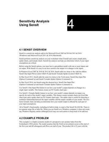
Where Ф0 and P0 are model output and parameter nominal values and Ф and P are themodel output and parameter values pertaining to a particular model run. An example ofthe sensen.txt file is presented in Example 7.2. Calculating Normalized Sensitivity Coefficient (NSC) Using MS ExcelThe normalized sensitivity coefficient (or sensitivity index) is calculated through thefollowing formula:NSC (Φ Φ 0 ) / Φ 0 Φ Φ 0 P0 ( P P0 ) / P0P P0 Φ 0(2)OrNSC Φ Φ0P P0 P0 Φ0 (3)Where, the NSC is a dimensionless positive number, whose value indicates the relativeimportance of parameter P on the model output Ф, that is, the relative sensitivity of theparticular model output Ф with respect to the changing of the particular model parameterP.The following steps illustrate how to calculate the NSC’s from the two SENSAN outputfiles (senabs.txt and sensen.txt) using MS Excel.Step 1: Create a new spreadsheet file named the current worksheet as surfacerunoff.6

Step 2: Using MS Excel File Import Wizard to open the senabs.txt file and copy the10 parameter names and their nominal values.Step 3: Place cursor in Cell A2 of surface runoff; right click and select PasteSpecial on the pop-up menu; and check the box in front of Transpose.7

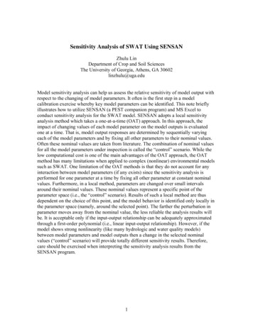
Step 4: The copied parameter names and their nominal values are pasted in surfacerunoff in a transposed manner.Step 5: To calculate the sensitivity of surface runoff with respect to the 10 SWATparameters, we give names for the columns as shown below.8

Step 6: From senabs.txt file we copy the “nominal” value of surface runoff (340.76mm).9

Step 7: Paste to the third column of surface runoff.xls.Step 8: Open sensen.txt file and copy the column of “runoff” starting from Row 3(omitting the first data line).10

Step 9: Paste to surface runoff.xls.Step 10: Calculate P0 / Φ 0 for surface runoff.11

Step 11: Calculate NSC (Equation 3).Step 12: Fill the rest row of the last two columns. Therefore, the last column contains thenormalized sensitivity coefficients of the 10 parameters with respect to surface runoff.12