Transcription
A quick guide to multisensi, an R package for multivariatesensitivity analysesCaroline Bidot, Hervé Monod, Marie-Luce TaupinMaIAGE, INRA, Université Paris-Saclay, 78350 Jouy-en-Josas, FranceApril 4, 2018Contents1 Introduction12 Case study: the Verhulst model of population dynamics23 Sequential univariate sensitivity analyses3.1 Calculation of sensitivity indices . . . . . . . . . . . . . . . . . . . . . . . . . . . .3.2 Graphical representation . . . . . . . . . . . . . . . . . . . . . . . . . . . . . . . . .3.3 Calculating simulations apart . . . . . . . . . . . . . . . . . . . . . . . . . . . . . .33454 Multivariate sensitivity analysis based on PCA4.1 Calculation . . . . . . . . . . . . . . . . . . . . . . . . . . . . . . . . . . . . . . . .4.2 Graphical representation . . . . . . . . . . . . . . . . . . . . . . . . . . . . . . . . .6685 Alternative reduction techniques5.1 Polynomial reduction of the multivariate output . . . . . . . . . . . . . . . . . . .5.2 Spline modelling of the population dynamics . . . . . . . . . . . . . . . . . . . . .1010126 Alternative methods of sensitivity analysis6.1 With Sobol2007 implemented in the package sensitivity . . . . . . . . . . . . . . . .6.2 With fast99 implemented in the package sensitivity . . . . . . . . . . . . . . . . . .1313151IntroductionGlobal sensitivity analysis is an essential tool for modellers in all application areas. Its aim isto quantify and compare the influence of uncertain parameters (or other input variables) on theoutput of a given model. There exist many different methods to perform sensitivity analysis, butthey are usually restricted to a single output variable. On the contrary, the R package multisensiis specifically designed to perform global sensitivity analyses on a multivariate model output. Itcalculates and represents graphically sensitivity indices on each output variable or on combinationsof output variables arising from dimension reduction techniques.The initial version of multisensi was based on the combination of (i) a factorial design on theuncertain model parameters; (ii) the application of principal components analysis on the modeloutput; (iii) anova-based sensitivity analyses on the first principal components. This idea wasproposed by Campbell et al. [1] and further studied by Lamboni et al. [5] (see also [11]). It is stillimplemented in multisensi, but the present version includes alternative methods to perform thedimension reduction : splines, bsplines and polynomial regression. In addition, several methods of1
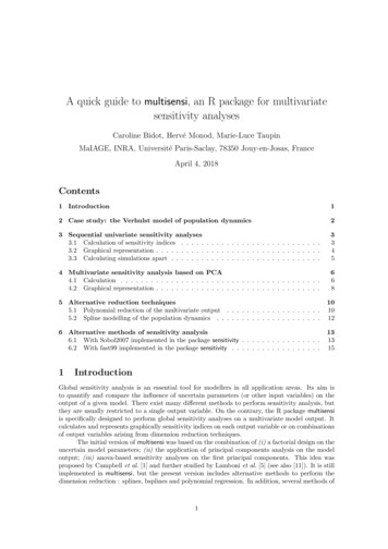
global sensitivity analysis can now be used, including those implemented in the package sensitivity[7].Applications in agronomy and epidemiology are presented by Lamboni et al. [4] and Luretteet al. [6]. For a detailed introduction to the methods of global sensitivity analysis, we refer toSaltelli et al. [9] and Faivre et al. [2] (in French). Multivariate techniques are presented, forexample, in James et al. [3].2Case study: the Verhulst model of population dynamicsIn the following, we illustrate the methods implemented in multisensi using a very simple model,the dynamic population model of Verhulst.Case study specifications The Verhulst model is given by the equationYt K,1 (K/Y0 1) exp( at)where Yt is the population size at time t and Y0 , K, a are respectively the initial size, the carryingcapacity and the rate of maximum population growth. The aim in our case study is to evaluatethe influence of these three parameters on the population sizes until time T 100. For this,simulated population sizes are recorded at times 5, 10, · · · , 100. The parameter uncertainty rangesof interest are assumed to be (100, 1000) for K, (1, 40) for Y0 , (0.05, 0.2) for a.Model implementation The R function verhulst is created to run the model for given valuesof K, a, Y0 and for a vector t of output times. The output of verhulst is the vector of populationsizes at the times in t.verhulst - function(K, Y0, a, t) {output - K/(1 (K/Y0 - 1) * exp(-a * t))return(output)}Since the methods implemented in multisensi require to run the dynamic population model repeatedly, another function called verhulst2 is created. It takes a dataframe of input combinations asits first argument and the time steps of interest as its second argument.T - seq(from 5, to 100, by 5)verhulst2 - function(X, t T) {out - matrix(nrow nrow(X), ncol length(t), NA)for (i in 1:nrow(X)) {out[i, ] - verhulst(X K[i], X Y0[i], X a[i], t)}out - as.data.frame(out)names(out) - paste("t", t, sep "")return(out)}A sample of population dynamics The output of the Verhulst model is plotted in Fig. 1, fora few combinations of values of the parameters.2
8006004002000Population sizen - 10set.seed(1234)X - data.frame(K runif(n, min 100, max 1000), Y0 runif(n, min 1,max 40), a runif(n, min 0.05, max 0.2))Y - verhulst2(X)par(cex.axis 0.7, cex.lab 0.8)plot(T, Y[1, ], type "l", xlab "Time", ylab "Population size",ylim c(0, 1000))for (i in 2:n) {lines(T, Y[i, ], type "l", col i)}20406080100TimeFigure 1: Population size versus time according to the Verhulst model for 10 combinations ofvalues of K, Y0 and a.33.1Sequential univariate sensitivity analysesCalculation of sensitivity indicesNow we want to perform sensitivity analyses on the population sizes with respect to the threeuncertain parameters: K, Y0 , and a. This can be done in different ways by using the mainfunction of the package, which is called multisensi like the package itself.A first and obvious option is to perform separate sensitivity analyses at t 5, 10, ., 100.To do this, multisensi must be used with the argument reduction NULL :library(multisensi)verhulst.seq - multisensi(model verhulst2, reduction NULL, center FALSE,design.args list( K c(100,400,1000), Y0 c(1,20,40), a c(0.05,0.1,0.2)))## [*] Design3
## [*] Response simulation## [*] Analysis Sensitivity IndicesBy keeping the default values of multisensi for the design and analysis arguments, a full factorialdesign is created according to the factors’ levels provided in the design.args argument. The resultsare then analysed by the R function aov, with an anova formula including main effects and twofactor interactions.The result verhulst.seq is an object of class dynsi, which has specific print, summary, and plotmethods. The print and summary functions give the sensitivity indices :print(verhulst.seq, digits 2)########################################Main sensitivity indicest5t10t15 t20K 0.014 0.053 0.096 0.13a 0.092 0.210 0.257 0.27Y0 0.818 0.519 0.335 0.24t60t65t70t75K 0.52 0.573 0.622 0.664a 0.18 0.165 0.146 0.128Y0 0.06 0.053 0.046 0.039Total sensitivityt5 t10 t15K 0.035 0.14 0.25a 0.148 0.35 0.45Y0 0.878 0.66 0.50t65 t70t75K 0.73 0.77 0.790a 0.32 0.29 0.259Y0 0.11 0.10 0.0913.2t25 t30 t35t40t45t50t550.18 0.23 0.30 0.351 0.393 0.433 0.4760.28 0.29 0.30 0.287 0.258 0.230 0.2060.20 0.16 0.12 0.087 0.073 0.068 0.064t80t85t90t95 t100GSI0.698 0.725 0.748 0.768 0.787 0.5620.111 0.096 0.082 0.069 0.058 0.1650.034 0.030 0.027 0.025 0.023 0.063indicest20 t25 t30 t35 t40 t450.34 0.41 0.48 0.55 0.59 0.610.49 0.49 0.50 0.51 0.51 0.480.40 0.33 0.25 0.18 0.15 0.14t80t85t90t95 t1000.808 0.822 0.832 0.842 0.8530.232 0.209 0.187 0.167 0.1480.086 0.083 0.082 0.081 0.079t50 t55 t600.64 0.67 0.700.44 0.40 0.360.14 0.13 0.13GSI0.710.320.13Graphical representationRather than reading tables of sensitivity indices, the user may prefer to plot them. Fig. 2 showsthe graphics obtained by the following code, where the two plot commands differ only by thenormalized argument :4
# color palettes: rainbow, heat.colors, terrain.colors, topo.colors,# cm.colorsplot(verhulst.seq, normalized TRUE, color terrain.colors, gsi.plot FALSE)title(xlab "Time in half-decades.")plot(verhulst.seq, normalized FALSE, color terrain.colors, gsi.plot FALSE)title(xlab "Time in .220000a0.0t25t50t75t100aresidualY0t25Time in half decades.t50t75t100Time in half decades.Figure 2: Dynamics of the sensitivity indices of the Verhulst model from t 5 to 100, with indicesnormalized either to 1 (left panel) or to the variance at each time t (right panel). In the left panel,the upper subplot shows the extreme (tirets), inter-quartile (grey) and median (bold line) outputvalues at all time steps. The lower subplot represents the sensitivity indices at all time steps forthe main effects and the first-order interactions.In the lower subplot of Fig. 2 (left panel), the sensitivity indices at time t are given bythe lengths of the different colors along the vertical bar at time t. Thus one can see clearlythat the population size at time t 25 is sensitive to the main effects of a, Y0 , K in quitesimilar proportions, with interactions accounting for roughly one-fourth of the variability. At timet 100, the population size is sensitive mainly to K, which is logical since the population sizes areclose to their carrying capacity K. The upper subplot illustrates how output quantiles vary alongthe time steps. This is useful to avoid over-interpretation of the sensitivity indices at times whenthe variability between simulations is low. For example, the population size is very sensitive to Y0in the first time steps, but then the variability between simulations is still very low as shown inthe upper subplot. This can also be seen by setting the argument normalized FALSE as in Fig. 2(right panel). In that case, the sensitivity indices at time t are constrained to sum to the outputvariance at time t rather than to reflect proportions summing to one at all times t.3.3Calculating simulations apartIf needed, the design or the model output can be calculated apart from the multisensi function.This allows to use a design generated outside multisensi or to apply multisensi to simulateddata based on a code implemented outside R. Thus, the commands below are equivalent to thosein Section 3.1 :X - expand.grid(K c(100,400,1000), Y0 c(1,20,40), a c(0.05,0.1,0.2))Y - verhulst2(X) ## this part can be performed outside R if necessaryverhulst.seq - multisensi(design X, model Y, reduction NULL, center FALSE)## [*] Analysis Sensitivity Indices5
4Multivariate sensitivity analysis based on PCAThe sequential sensitivity analyses of Section 3 give interesting information on the evolution ofparameters’ influence over time. However other methods based on multivariate techniques cangive a more synthetic view of the parameters’ impact on the population dynamics. Their commonprinciple is to proceed to the analysis in two steps:1. dimension reduction: a multivariate technique is applied to decompose the simulateddynamics on a reduced basis of d canonical dynamics, which will be called the basic trajectories. The multivariate techniques available in multisensi are principal components analysis(PCA), B-splines, orthogonal B-splines or projection on a polynomial basis;2. sensitivity analysis: for each basic trajectory, sensitivity analysis is applied to the associated coefficients of the decomposition.Mathematically, the population dynamics are decomposed intoYi,t dXαij Zj,t ηi,t ,(1)j 1 where Yi,t is the output of simulation i at time t, Zj,t t 1,··· ,T is the jth basic trajectory (whichdepends on the multivariate technique), αij is the coefficient of simulation i associated with thejth basic trajectory, d is the reduction dimension and ηi,t is the approximation error on simulationi at time t due to dimension reduction. Sensitivity analyses are applied to the αij coefficients,for each basic dimension j 1, · · · , d. In addition, it is possible to calculate the generalisedsensitivity indices (GSI), which are weighted means of the sensitivity indices over the d dimensions,and the global criterion (GC), which quantifies the proportion of variability accounted for bythe approximation resulting from both the dimension reduction and the restriction to low-orderfactorial effects in the sensitivity analysis (see Lamboni et al. [5] and [11]).In this Section, we illustrate this approach by focusing on principal components analysis(PCA). For any given reduced dimension d, the PCA decomposition maximises the variabilitybetween dynamics taken into account by the summation in equation (1). Let V denote thevariance-covariance matrix of the T vectors of simulated output variables Yi,t i 1,··· ,N , where N is the size of the design; then the PCA basic trajectories Zj,t t 1,··· ,T are the eigenvectors of Vin decreasing order of their associated eigenvalues.4.1CalculationMultivariate sensitivity analyses can be performed by using the same multisensi function as before.The choice of the multivariate technique is now specified by the argument reduction basis.ACP :## Note that this old syntax of multisensi still works:## verhulst.gsi - gsi(formula 2, Y, X)verhulst.pca - multisensi(design X, model Y, reduction basis.ACP, scale FALSE)## [*] Dimension Reduction## [*] Analysis Sensitivity Indices## [*] Goodness of fit computing6
By keeping the default argument dimension 0.95, the dimension d is selected automatically asthe smallest value such that 95% of the total variability (or inertia) between dynamics is taken intoaccount. Another option would be to specify dimension 3, for example. Two other argumentsare associated with dimension reduction, center and scale. When the output is a time series withthe same variable calculated from time t 1 to t T , as in our Verhulst model case study, itcan be more pertinent to keep the raw ranges of variation of Y over time. This is why we use theargument scale FALSE. Note that we choose to use again the factorial design X and the simulatedoutput Y calculated in Section 3.3. By default, the sensitivity analyses are performed by anovawith a formula including main effects and two-factor interactions, as in Section 3.The result verhulst.pca is an object of class gsi, which has print, summary and plot methodsassociated, in addition to the more specific functions graph.pc and graph.bar. The summary givesinformation on the inertia proportions explained by the first principal components, together withthe tables of sensitivity indices.summary(verhulst.pca, digits ########Components cumulated inertia percentages and Global CriterionPC1 PC2 GC90 98 96Main sensitivity indicesPC1 PC2GSIK 0.610 0.15 0.573a 0.159 0.27 0.168Y0 0.059 0.10 0.063Total sensitivity indicesPC1 PC2 GSIK 0.76 0.33 0.73a 0.29 0.59 0.32Y0 0.11 0.30 0.12gsi outputsDesign"X"Loadings"L"First order "Response Principal Components"Y""H"PCs variancesIndices"lambda""SI"Total indices Interaction ere the inertia proportions show that the first two principal components explain 98%of the total variability between the calculated population dynamics. So by default, the multisensifunction performs the sensitivity analyses for these first two components only. The first componentis influenced mainly by K (SI 0.61), while the second component is influenced mainly by a,although less strongly. The influence of Y0 is exerted mainly through interactions with K and a.The last column in the tables of sensitivity indices gives the generalised sensitivity indices (GSI),which are the averages of the PC1 and PC2 indices weighted by the PC percentages of inertia.7
4.2Graphical representationWhen a reduction technique is applied, several types of graphical representation can be useful tointerpret the results. This is why the plot method allows for several options to be used dependingon the value given to the graph argument.The graph 1 option gives multipanel graphics as shown in Fig. 3. There is one column perdimension j and two rows. The aim of the upper row is to show what the components in dimension j look like with respect to the output variables, so they present quantile curves αQj Zj,t t 1,··· ,T ,where αQj denotes the quantile Q of the αij values for i 1, · · · , N (see details in the legend ofFig. 3). The lower row contains the bar plot of sensitivity indices for each dimension j of interest.plot(verhulst.pca, graph 1)PC2 (7.93 %) 300 200 0 100200100600300PC1 (90.2 .4t1000.3t750.2t500.1t25SIFigure 3: Plots for the PCA multivariate sensitivity analysis of the Verhulst model. Upper subplots: functional boxplots of the principal components, with time on the x-axis and populationsize contribution on the y-axis (red curves: extreme values, blue: 1/10 and 9/10 percentiles, greyarea: inter-quartile, black: median). Lower subplots: sensitivity indices (light grey: first orderindices, dark grey: total indices).For the Verhulst case study, the left upper plot in Fig. 3 shows that the first principalcomponent, which explains more than 90% of the inertia, captures essentially an average effect8
over time. The left lower plot confirms that this effect is mainly influenced by the maximumpopulation size K, with smaller contributions of a, Y0 and interactions.The right upper plot in Fig. 3 shows that the second principal component, which explainsabout 8% of the inertia, captures the contrast in the dynamics between the early and late periods.The right lower plot shows that this effect is influenced first by a, but also by K and Y0 and bystrong two-factor interactions.The graph 2 option gives the bar plot of generalised sensitivity indices (see Fig. 4). In thecase study, these indices represent the contributions of the factors to the whole variability betweenthe dynamics of population size.plot(verhulst.pca, graph 2)Ka0.60.40.20.0Y0GSIFigure 4: Bar plot of the PCA generalised sensitivity indices of the Verhulst model.For each output variable, the multivariate sensitivity analysis accounts only for part ofthe variability between simulations. The first reason is due to dimension reduction. The secondreason is because the sensitivity analysis is usually restricted to the factorial effects of first orderor possibly first and second order. In multisensi, these proportions of variability that are accountedfor can be quantified by R2 coefficients of determination, provided the sensitivity analysis is basedon anova. The graph 3 option allows to plot these R2 coefficients of determination, as shownin Fig. 5 for the case study. The R2 values are low for the first output variables, because theyhave low variance and so have little weight in the determination of the basic trajectories. TheR2 values would have been more uniform if we had chosen to normalise the output variables bysetting scale TRUE.9
0.60.40.00.2Rsquare0.81.0plot(verhulst.pca, graph 3)5101520IndexFigure 5: Coefficients of determination of the output variables for the PCA multivariate sensitivityanalysis of the Verhulst model on raw output data.5Alternative reduction techniquesIn practice, it can be useful to apply sensitivity analysis with multivariate techniques other thanPCA. The package multisensi provides projection methods either on a reduced polynomial basisor on data-based spline bases.5.1Polynomial reduction of the multivariate outputIn the case of a polynomial decomposition, the (Yi,t )t 1,··· ,T dynamics are approximated by polynomials of a given degree d 1. Thus the (Zj,t )t 1,··· ,T basic trajectories of equation (1) are themonomials of t of degree up to d 1.In multisensi, this decomposition is obtained by setting the argument reduction basis.poly.It is necessary to give additional information through the basis.args argument. We do it here forthe Verhulst model by specifying that the polynomial must be of degree six or lower and by givingthe vector of output time coordinates t (5, · · · , 100)T .verhulst.poly - multisensi(design X, model Y, reduction basis.poly,dimension 0.99, center FALSE, scale FALSE, cumul FALSE,basis.args list(degree 6, x.coord T), analysis analysis.anoasg,analysis.args list(formula 2, keep.outputs FALSE))## [*] Dimension Reduction## [*] Analysis Sensitivity Indices## [*] Goodness of fit computingsummary(verhulst.poly, digits 2)10
######Components cumulated inertia percentages and Global CriterionDeg0 Deg1 Deg2 Deg3GC7693989997Main sensitivity indicesDeg0Deg1 Deg2Deg3GSIK 0.571 0.7327 0.093 0.0047 0.567a 0.179 0.0526 0.331 0.2838 0.166Y0 0.078 0.0014 0.049 0.0902 0.064Total sensitivity indicesDeg0 Deg1 Deg2 Deg3 GSIK 0.73 0.79 0.39 0.22 0.72a 0.31 0.20 0.71 0.64 0.32Y0 0.12 0.10 0.21 0.32 0.13gsi outputsDesign"X"Loadings"L"First order "Response Principal Components"Y""H"PCs variancesIndices"lambda""SI"Total indices Interaction he results show that polynomials of degree 3 are sufficient to integrate more than 99% ofthe output variability. Graphics are given in Fig. 6.11
plot(verhulst.poly, nb.comp 3, graph 1)Deg1 (16.8 %)Deg2 (5.14 %)200100 300 200 0 600200 20040000200600400800600Deg0 (76.1 %)SIFigure 6: Plots for the multivariate sensitivity analysis based on polynomial regression. Uppersubplots: functional boxplots of the constant, linear and quadratic components, with time on thex-axis and population size contribution on the y-axis (red curves: extreme values, blue: 1/10 and9/10 percentiles, grey area: inter-quartile, black: median). Lower subplots: sensitivity indices(light grey: first order indices, dark grey: total indices).5.2Spline modelling of the population dynamicsSplines represent other popular techniques of multivariate analysis (see [3, 10, 8]). We give anexample just below with B-splines, see also Fig. 7. More information is given in the help ofbasis.bsplines.## bsplinesverhulst.bspl - multisensi(design X, model Y, reduction basis.bsplines,dimension NULL, center FALSE, scale FALSE,basis.args list(knots 10, mdegree 3), cumul FALSE,analysis analysis.anoasg,analysis.args list(formula 2, keep.outputs FALSE))## [*] Dimension Reduction## [*] Analysis Sensitivity Indices## [*] Goodness of fit computing12
plot(verhulst.bspl, nb.comp 5, graph 1)B8 (6.01 K0.6K0.4K0.2K0.0KSIt50t75t1000.6t500.5t250100 200 300 400 500100 200 300 400 500t1000.4t750.3t500.2t250.1t1000.0t75B6 (5.22 %)00t500100 200 300 400 500 6008006004002000t25B7 (5.78 %)100 200 300 400 500 600B9 (6.24 %)1000B13 (7.81 %)SIFigure 7: Plots for the multivariate sensitivity analysis based on bspline regression. Upper subplots: functional boxplots of the b-splines, with time on the x-axis and population size contribution on the y-axis (red curves: extreme values, blue: 1/10 and 9/10 percentiles, grey area:inter-quartile, black: median). Lower subplots: sensitivity indices (light grey: first order indices,dark grey: total indices).6Alternative methods of sensitivity analysisSensitivity analyses based on factorial design plus anova are very useful and convenient. However,they oblige to restrict the levels of each input factor to a few discretised values from their uncertainty ranges. Other methods of global sensitivity analysis take better account of continuousranges of input values. Many of them can be used with multisensi.6.1With Sobol2007 implemented in the package sensitivityThe function multisensi is compatible with the methods of sensitivity analysis implemented in thesensitivity package. To illustrate this, we first call the sensitivity package:library(sensitivity)Then we use the method sobol2007 of the sensitivity package :m - 10000Xb - data.frame(K runif(m, min 100, max 1000), Y0 runif(m, min 1,max 40), a runif(m, min 0.05, max 0.2))verhulst.seq.sobol - multisensi(design sobol2007, model verhulst2,reduction NULL, analysis analysis.sensitivity, center TRUE,design.args list(X1 Xb[1:(m/2), ], X2 Xb[(1 m/2):m, ], nboot 100),analysis.args list(keep.outputs FALSE))## [*] Design## [*] Response simulation## [*] Analysis Sensitivity Indicesprint(verhulst.seq.sobol, digits 2)####Main sensitivity indices13
####################################t5t10t15 t20K 0.0093 0.031 0.069 0.12a 0.1075 0.280 0.386 0.43Y0 0.8405 0.581 0.393 0.27t60t65t70t75K 0.735 0.790 0.835 0.871a 0.141 0.107 0.079 0.058Y0 0.023 0.017 0.013 0.009t25 t30 t35t40t450.19 0.26 0.34 0.429 0.5130.43 0.40 0.37 0.322 0.2740.20 0.14 0.10 0.073 0.054t80t85t90t950.8984 0.920 0.9359 0.94800.0412 0.029 0.0201 0.01380.0062 0.004 0.0024 0.0013t50 t550.59 0.670.23 0.180.04 0.03t100GSI0.9568 0.7040.0094 0.1530.0005 0.042Total sensitivity indicest5t10 t15 t20 t25 t30 t35 t40t45t50t55K 0.013 0.061 0.14 0.23 0.33 0.42 0.50 0.58 0.650 0.714 0.771a 0.152 0.380 0.52 0.58 0.58 0.55 0.51 0.45 0.391 0.329 0.269Y0 0.877 0.671 0.50 0.36 0.26 0.19 0.14 0.10 0.082 0.068 0.056t60 t65t70t75t80t85t90t95 t100GSIK 0.818 0.86 0.890 0.916 0.936 0.952 0.963 0.972 0.979 0.783a 0.214 0.17 0.128 0.096 0.071 0.051 0.037 0.026 0.017 0.222Y0 0.047 0.04 0.034 0.028 0.024 0.020 0.016 0.013 0.010 0.068Results are given above and the sequence of sensitivity indices is displayed in Fig. 8. Theresults are very similar to those of Section 3, but here they have obtained by varying the inputfactors across their whole uncertainty intervals.Of course, the Sobol method of sensitivity analysis can also be combined with the multivariate techniques (PCA, polynomials, splines), by changing the reduction argument.14
plot(verhulst.seq.sobol, normalized TRUE, color terrain.colors, gsi.plot FALSE)title(xlab "Time in 0.6Ka0.40.2Y00.0t25t50t75t100Time in half decadesFigure 8: Evolution of the Sobol sensitivity indices of the Verhulst model from t 5 to t 100.The upper subplot shows the extreme (tirets), inter-quartile (grey) and median (bold line) outputvalues at all time steps. The lower subplot represents the sensitivity indices at all time steps forthe main effects and the first-order interactions.6.2With fast99 implemented in the package sensitivityAnother possibility is to use the method fast99 :verhulst.seq.fast - multisensi(design fast99, model verhulst2,center FALSE, reduction NULL, analysis analysis.sensitivity,design.args list( factors c("K","Y0","a"), n 1000, q "qunif",q.arg list(list(min 100, max 1000), list(min 1, max 40),list(min 0.05, max 0.2))),analysis.args list(keep.outputs FALSE))## [*] Design## [*] Response simulation## [*] Analysis Sensitivity Indicesprint(verhulst.seq.fast,digits 2)#### Main sensitivity indices##t5t10 t15 t20 t25 t30t35t40t45t50t55## K 0.0047 0.024 0.06 0.11 0.18 0.26 0.346 0.435 0.522 0.603 0.67615
################################a 0.1094 0.286 0.40 0.45 0.45 0.43 0.391 0.341Y0 0.8507 0.597 0.40 0.28 0.20 0.14 0.096 0.068t60t65t70t75t80t85t90K 0.74 0.797 0.843 0.8809 0.9110 0.9345 0.9523a 0.14 0.109 0.081 0.0581 0.0410 0.0284 0.0194Y0 0.02 0.015 0.011 0.0083 0.0061 0.0044 0.0031Total sensitivity indicest5t10 t15 t20 t25 t30 t35 t40K 0.011 0.056 0.14 0.23 0.32 0.41 0.50 0.57a 0.141 0.364 0.51 0.57 0.58 0.57 0.53 0.48Y0 0.884 0.675 0.50 0.36 0.26 0.19 0.14 0.11t60t65t70t75t80t85t90K 0.817 0.859 0.893 0.921 0.942 0.959 0.971a 0.236 0.187 0.146 0.113 0.086 0.065 0.049Y0 0.061 0.054 0.047 0.041 0.035 0.029 0.0240.287 0.234 0.1860.049 0.036 0.027t95t100GSI0.9657 0.9755 0.7140.0130 0.0085 0.1590.0022 0.0015 .7850.2390.076Results are shown above and the sequence of sensitivity indices is displayed in Fig. 9.plot(verhulst.seq.fast, normalized TRUE, color terrain.colors, gsi.plot FALSE)title(xlab "Time in 0.6Ka0.40.2Y00.0t25t50t75t100Time in half decadesFigure 9: Evolution of the Fast sensitivity indices of the Verhulst model from t 5 to t 100.The upper subplot shows the extreme (tirets), inter-quartile (grey) and median (bold line) outputvalues at all time steps. The lower subplot represents the sensitivity indices at all time steps forthe main effects and the first-order interactions.16
AcknowledgementsThis document was typed using the knitr package ([12, 13]).References[1] K. Campbell, M. McKay & B. Williams – “Sensitivity analysis when model outputs arefunctions”, Reliability Enineering and Systems Safety 91 (2006), p. 1468–1472.[2] R. Faivre, B. Iooss, S. Mahévas, D. Makowski & H. Monod (éds.) – Analyse de sensibilité et exploration de modèles. applications aux sciences de la nature et de l’environnement,Collection Savoir-Faire. Éditions Quae, 2013.[3] G. James, D. Witten, T. Hastie & R. Tibshirani (éds.) – An introduction to statisticallearning with applications in R, Springer Texts in Statistics, Springer, 2013.[4] M. Lamboni, D. Makowski, S. Lehuger, B. Gabrielle & H. Monod – “Multivariateglobal sensitivity analysis for dynamic crop models”, Field Crops Research 113 (2009), p. 312–320.[5] M. Lamboni, H. Monod & D. Makowski – “Multivariate sensitivity analysis to measureglobal contribution of input factors in dynamic models”, Reliability Engineering & SystemSafety 96 (2011), p. 450–459.[6] A. Lurette, S. Touzeau, M. Lamboni & H. Monod – “Sensitivity analysis to identify keyparameters influencing Salmonella infection dynamics in a pig batch”, Journal of TheoreticalBiology 258 (2009), no. 1, p. 43–52.[7] G. Pujol, B. Iooss & A. Janon – “Package ‘sensitivity’. a collection of functions for factorscreening, global sensitivity analysis and reliability sensitivity analysis of model output”,Tech. Report Version 1.11.1, 2015, with contributions from Sebastien Da Veiga, Jana Fruth,Laurent Gilquin, Joseph Guilla
global sensitivity analysis can now be used, including those implemented in the package sensitivity [7]. Applications in agronomy and epidemiology are presented by Lamboni et al. [4] and Lurette et al. [6]. For a detailed introduction to the methods of global sensitivity analysis, we refer to Saltelli et al. [9] and Faivre et al. [2] (in French).