Transcription
Abaqus/CFD – Sample ProblemsAbaqus 6.10
Contents1.2.3.4.5.6.Oscillatory Laminar Plane Poiseuille FlowFlow in Shear Driven CavitiesBuoyancy Driven Flow in CavitiesTurbulent Flow in a Rectangular ChannelVon Karman Vortex Street Behind a Circular CylinderFlow Over a Backward Facing StepThis document provides a set of sample problems that can be usedas a starting point to perform rigorous verification and validationstudies. The associated Python scripts that can be used to createthe Abaqus/CAE database and associated input files are provided.2
1.Oscillatory Laminar Plane PoiseuilleFlow
Oscillatory Laminar Plane Poiseuille FlowOverviewThis example compares the prediction of the time-dependent velocity profile in a channelsubjected to an oscillatory pressure gradient to the analytical solution.Problem descriptionA rectangular 2-dimensional channel of width 1m and length 2m is considered. Anoscillatory pressure gradient (with zero mean) is imposed at the inlet. The analysis is carriedout in two steps. In the first analysis step, a constant pressure gradient is prescribed for thefirst 5 seconds of the simulation to initialize the velocity field to match that of the analyticalsteady-state solution. In the second analysis step, the flow is subjected to an oscillatorypressure gradient. A 40x20 uniform mesh is used for this problem. Two dimensionalgeometry is modeled as three dimensional with one element in thickness direction.Wall boundary condition1mTime-dependent inlet pressurezxWall boundary condition2mOutletdP P0 cos( (t to ))dxSchematic of the geometry usedInlet pressure profile
Oscillatory Laminar Plane Poiseuille FlowFeaturesLaminar flowTime-dependent pressure inletMulti-step analysisBoundary conditionsPressure inlett to : p 7.024t to : p 10*Cos( (t-to)) ; to 5, p/5Pressure outlet (p 0)No-slip wall boundary condition on top and bottom (V 0)Analytical solutiondP P0 e i tdx Po 2s i t cos( z h) u ( y, t ) Re e 1 cos( h) 2i References i s h is the half-channel widthPo is the amplitude ofpressure gradient oscillation is the circular frequency2 Fluid Mechanics, Second Edition: Volume 6 (Course of Theoretical Physics), Authors: L. D. Landau,E.M. Lifshitz5
Oscillatory Laminar Plane Poiseuille FlowResultsT 5 secVelocity profile: Comparison with analytical solutionT 10 secFilesex1 oscillatory planeflow.pyex1 oscillatory planeflow mesh.inp6
2. Flow in Shear Driven Cavities7
Flow in Shear Driven CavitiesOverviewThis sample problem compares the prediction of velocity profiles in shear-driven cavities ofdifferent shapes. 2-dimensional 900, 450 and 150 cavities are considered. Shear driven flowin a cubical box is also presented. Velocity profiles in each of these cases are comparedagainst numerical results available in literature.Problem descriptionThe following cavity configurations and Reynolds’ numbers are presented1m1m1m1m1m(a) 900 Cavity1m(b) 450 Cavity1m(c) 150 Cavity900 Cavity: Reynolds number 100, 3200; Mesh: 129x129x1450 Cavity: Reynolds number 100; Mesh: 512x512x1150 Cavity: Reynolds number 100; Mesh: 256x256x1Cubical box: Reynolds number 400; Mesh: 32x32x321m1m(d) Cubical box
Flow in Shear Driven CavitiesFeaturesLaminar shear driven flowBoundary conditionsSpecified velocity at top plane to match flow Reynolds’ numberNo-slip at all other planes (V 0)Hydrostatic mode is eliminated by setting reference pressure to zero at a single nodeReferences1.“High-Re Solutions for Incompressible Flow Using the Navier-Stokes Equations and a Multigrid Method”U. Ghia, K. N. Ghia, and C. T. ShinJournal of Computational Physics 48, 387-411 (1982)2.“Numerical solutions of 2-D steady incompressible flow in a driven skewed cavity”Ercan Erturk and Bahtiyar DursunZAMM · Z. Angew. Math. Mech. 87, No. 5, 377 – 392 (2007)3."Flow topology in a steady three-dimensional lid-driven cavity"T.W.H. Sheu, S.F. Tsai, Computers & Fluids, 31, 911–934 (2002)9
Flow in Shear Driven Cavities900 CavityResultsVelocities along horizontal and vertical centerlinesRe 100Re 320010
Flow in Shear Driven CavitiesSkew Cavity (450 and 150)ResultsVelocities along horizontal and vertical centerlines45015011
Flow in Shear Driven CavitiesCubical BoxResultsVelocity vectorsVelocities along horizontal and vertical centerlines12
Flow in Shear Driven CavitiesFilesex2 sheardriven cavity.pyex2 cavity15deg mesh.inpex2 cavity45deg mesh.inpex2 cubicalbox mesh.inpex2 sqcavity mesh.inp13
3. Buoyancy Driven Flow inCavities14
Buoyancy Driven Flow in CavitiesOverviewThis sample problem compares the prediction of velocity profiles due to buoyancy driven flowin square and cubical cavities. The cavities are differentially heated to obtain a temperaturegradient. Velocity profiles in each of these cases are compared against numerical resultsavailable in the literature.Problem descriptionThe material properties are chosen to match the desired Rayleigh number, RaRa q 0.0g L3 T , Kinematic viscosity , Thermal diffusivity , Thermal expansion coefficientg, Acceleration due to gravityT 1.0T 0.0x 0, T 1.0q 0.0Square Cavity: Rayleigh number 1e3, 1e6Cubical Cavity: Rayleigh number 1e4x 1.0, T 1.0All other faces areadiabatic
Buoyancy Driven Flow in CavitiesFeaturesBuoyancy driven flowBoussinesq body forcesBoundary conditionsNo-slip velocity boundary condition on all the planes (V 0)Specified temperaturesHydrostatic mode is eliminated by setting reference pressure to zero at a single nodeReferences1.“Natural Convection in a Square Cavity: A Comparison Exercise”G. de Vahl Davis and I. P. JonesInternational Journal for Numerical Methods in Fluids, 3, 227-248, (1983)2."Benchmark solutions for natural convection in a cubic cavity using the high-order time–space method"Shinichiro Wakashima, Takeo S. SaitohInternational Journal of Heat and Mass Transfer, 47, 853–864, (2004)16
Buoyancy Driven Flow in Cavities2D Square e Vahl Davis)u3.6953.697x0.17810.178PresentBenchmark(de Vahl Davis)u3.6543.649x0.81290.813PresentBenchmark(de Vahl Davis)q 0.0T 1.0T 0.0q 0.0Ra 1000, Pr 0.71TemperatureVelocityPresentBenchmark(de Vahl 85Ra 1.0e6 , Pr 0.7117
Buoyancy Driven Flow in CavitiesCubical BoxResultsRa 1.0e4, Pr 0.71 2 (0,0,0) U1 (0.5,0.5, z ) U 3 ( x,0.5,0.5)maxmaxBenchmark(Wakashima &Saitoh (2004))1.10180.1984(z 0.8250)0.2216(x %0.2%PresentBenchmarkTemperature contours at the mid plane(y 0.5)PresentBenchmarkVorticity contours at the mid plane (y 0.5)18
Buoyancy Driven Flow in CavitiesFilesex3 buoyancydriven flow.pyex3 sqcavity mesh.inpex3 cubicbox mesh.inp19
4. Turbulent Flow in aRectangular Channel20
Turbulent Flow in a Rectangular ChannelOverviewThis example models the turbulent flow in a rectangular channel at a friction Reynoldsnumber 180 and Reynolds number (based on mean velocity) 5600. The one equationSpalart-Allmaras turbulence model is used. The results are compared with direct numericalsimulation (DNS) results available in the literature as well as experimental results.Abaqus/CFD results at a friction Reynolds number 395 and Reynolds number (based onmean velocity) 13750 are also presented.Problem descriptionA rectangular 2-dimensional channel of width 1 unit and length 10 units is considered. Apressure gradient is imposed along the length of the channel by means of specified pressureat the inlet and zero pressure at the outlet. The pressure gradient is chosen to impose thedesired friction Reynolds number for the flow.Wall boundary conditionInletOutletH 1Wall boundary conditionL 10
Turbulent Flow in a Rectangular ChannelProblem description (cont’d)The Reynolds number is defined as Re rUavH/mThe friction Reynolds number is defined as Ret rut(H/2)/m , where ut is the frictionvelocity defined asut twrtw wall shear stressFeaturesTurbulent flowSpalart-Allmaras turbulence modelBoundary conditionsNo-slip velocity boundary condition on channel walls(V 0)Set through thickness velocity components to zeroDistance function 0, Kinematic turbulent viscosity 0 at No-slip velocity boundary conditionMeshMesh – 50 (Streamwise) X 91 (Normal) X 1 (Through thickness)y at first grid point 0.04622
Turbulent Flow in a Rectangular ChannelReferences1.2.“Turbulence statistics in fully developed channel flow at low Reynolds number”J. Kim, P. Moin and R. MoserJournal of Fluid Mechanics, 177, 133-166, (1987)“The structure of the viscous sublayer and the adjacent wall region in a turbulent channel flow”H. EckelmannJournal of Fluid Mechanics, 65, 439, (1974)23
Turbulent Flow in a Rectangular ChannelResults“Law of the wall”u U ut y,y ut Results are presented at Ret 180Abaqus/CFD results at Ret 395 isalso presented24
Turbulent Flow in a Rectangular ChannelResultsVelocity profile25
Turbulent Flow in a Rectangular ChannelFilesex4 turb channelflow.pyex4 turb channelflow mesh.inpNoteAbaqus/CFD results at a friction Reynolds number 395 and Reynolds number(based on mean velocity) 13750 can be obtained by setting a pressuregradient of 0.057326
5. Von Karman Vortex StreetBehind a Circular Cylinder27
Von Karman Vortex Street Behind a Circular CylinderOverviewThis example simulates the Von Karman vortex street behind a circular cylinder at a flowReynolds number of 100 based on the cylinder diameter. The frequency of the vortexshedding is compared with results available in the literature.Problem descriptionThe computational domain for the vortex shedding calculations consists of an interior squareregion (-4 x 4; -4 y 4) surrounding a cylinder of unit diameter. The domain isextended in the wake of cylinder up to x 20 unitsInletD 1OutletH 8“Tow-tank” conditionH 20
Von Karman Vortex Street Behind a Circular CylinderFeaturesUnsteady laminar flowReynolds number rUinlet D/mFluid PropertiesDensity 1 unitViscosity 0.01 unitsBoundary conditionsTow tank condition at top and bottom walls:U 1, V 0Inlet velocity: Uinlet 1, V 0Set through thickness velocity components to zeroOutlet: P 0Cylinder surface: No-slip velocity boundary condition (V 0)29
Von Karman Vortex Street Behind a Circular CylinderReferences1.Transient flow past a circular cylinder: a benchmark solution”,M. S. Engelman and M. A. JamniaInternational Journal for Numerical Methods in Fluids, 11, 985-1000, (1990)30
Von Karman Vortex Street Behind a Circular CylinderResultsTotal numberof elementStrouhal Number* tCoarse17600.17490.03Fine281600.17350.0075*St fD/Uinlet , f is the frequency of vortex sheddingThe results are consistent with the Strouhal numbers reported in the reference(0.172-0.173)The frequency of the vortex shedding is obtained as the half of the peak frequencyobtained by a FFT of kinetic energy plot (from t 200 sec to 300 sec)31
Von Karman Vortex Street Behind a Circular CylinderResultsKinetic energy32
Von Karman Vortex Street Behind a Circular CylinderResultsVelocity contour plot at t 300 secPressure line plot at t 300 sec33
6. Flow Over a BackwardFacing Step34
Flow Over a Backward Facing StepOverviewThis example simulates the laminar flow over a backward facing step at a Reynolds numberof 800 based on channel height. The results are compared with numerical as well asexperimental results available in literature.Problem descriptionThe computational domain for the flow calculations consists of an rectangular region (0 x 30; -0.5 y 0.5). The flow enters the solution domain from 0 y 0.5 while -0.5 y 0.0represents the step. A parabolic velocity profile is specified at the inlet.No-slipVx(y) 24y(0.5 – y)Vav 1.0OutletP 0H 1No-slipNo-slipL 30Re rVav Hm
Flow Over a Backward Facing StepFeaturesSteady laminar flowFluid PropertiesDensity 1 unitViscosity 0.00125 units (the viscosity is chosen so as to set the flow Reynoldsnumber to 800)Boundary conditionsSet through thickness velocity components to zeroNo-slip velocity boundary condition at top and bottom wallsVx 0, Vy 0Inlet velocity: Parabolic velocity profile - Vx f(y)Vy 0Outlet: P 0No-slip velocity boundary condition at the step boundaryVx 0, Vy 036
Flow Over a Backward Facing StepReferences“A test problem for outflow boundary conditions – Flow over a backward-facing step”D. K. Gartling, International Journal for Numerical Methods in FluidsVol 11, 953-967, (1990)37
Flow Over a Backward Facing StepResultsL3L2L1Zone 1 (0 x 15)Uniform mesh x, yZone 2 (15 x 30)Graded mesh x 2 x, y constantMesh(Across the channel x alongthe channel length)L1Length from the step face to thelower re-attachment pointL2Length from the stepface to upperseparation pointL3Length of the upperseparation bubbleGartling (1990)40x8006.14.8510.48Abaqus/CFDFine80x1200x1 (Zone 1)80x832x1 (Zone 2)5.99194.911310.334Abaqus/CFDMedium40x600x1 (Zone 1)40x416x1 (Zone 2)5.74714.837910.101Abaqus/CFDCoarse20x300x1 (Zone 1)20x208x1 (Zone 2)4.50183.96598.7748Elements used by Gartling (1990) were biquadratic in velocity and linear discontinuous pressure elements. Incontrast, the fluid elements in Abaqus/CFD use linear discontinuous in velocity and linear continuous inpressure.38
Flow Over a Backward Facing StepResultsPressure line plot (0 x 30)Velocity line plot (0 x 15)Out of plane vorticity (0 x 30)39
Flow Over Backward Facing StepResultsHorizontal velocity at x 7 & x 1540
Flow Over Backward Facing StepResultsVertical velocity at x 7 & x 1541
Flow Over Backward Facing StepFilesex6 backwardfacingstep.pyex6 backwardfacingstep coarse.inpex6 backwardfacingstep medium.inpex6 backwardfacingstep fine.inpcoarse parabolic inlet velocity.inpmedium parabolic inlet velocity.inpfine parabolic inlet velocity.inpNoteThe models require a parabolic velocity profile at the inlet. This needs to bemanually included as boundary condition in the generated input file.The parabolic velocity profile required is provided in filescoarse parabolic inlet velocity.inp, medium parabolic inlet velocity.inp andfine parabolic inlet velocity.inp for coarse, medium and fine meshes,respectively.42
number 180 and Reynolds number (based on mean velocity) 5600. The one equation Spalart-Allmaras turbulence model is used. The results are compared with direct numerical simulation (DNS) results available in the literature as well as experimental results. Abaqus/CFD results at a friction Reynolds number 395 and Reynolds number (based on