Transcription
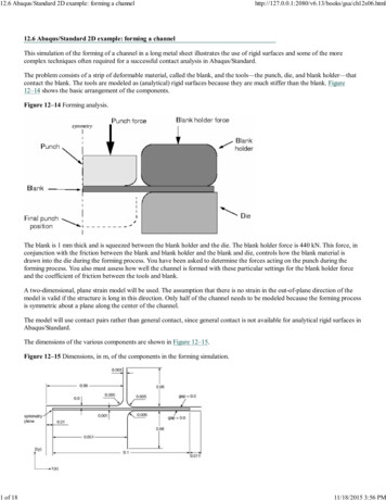
12.6 Abaqus/Standard 2D example: forming a channel1 of ml12.6 Abaqus/Standard 2D example: forming a channelThis simulation of the forming of a channel in a long metal sheet illustrates the use of rigid surfaces and some of the morecomplex techniques often required for a successful contact analysis in Abaqus/Standard.The problem consists of a strip of deformable material, called the blank, and the tools—the punch, die, and blank holder—thatcontact the blank. The tools are modeled as (analytical) rigid surfaces because they are much stiffer than the blank. Figure12–14 shows the basic arrangement of the components.Figure 12–14 Forming analysis.The blank is 1 mm thick and is squeezed between the blank holder and the die. The blank holder force is 440 kN. This force, inconjunction with the friction between the blank and blank holder and the blank and die, controls how the blank material isdrawn into the die during the forming process. You have been asked to determine the forces acting on the punch during theforming process. You also must assess how well the channel is formed with these particular settings for the blank holder forceand the coefficient of friction between the tools and blank.A two-dimensional, plane strain model will be used. The assumption that there is no strain in the out-of-plane direction of themodel is valid if the structure is long in this direction. Only half of the channel needs to be modeled because the forming processis symmetric about a plane along the center of the channel.The model will use contact pairs rather than general contact, since general contact is not available for analytical rigid surfaces inAbaqus/Standard.The dimensions of the various components are shown in Figure 12–15.Figure 12–15 Dimensions, in m, of the components in the forming simulation.11/18/2015 3:56 PM
12.6 Abaqus/Standard 2D example: forming a channel2 of ml12.6.1 Preprocessing—creating the model with Abaqus/CAEUse Abaqus/CAE to create the model. Abaqus provides scripts that replicate the complete analysis model for this problem. Runone of these scripts if you encounter difficulties following the instructions given below or if you wish to check your work.Scripts are available in the following locations:A Python script for this example is provided in “Forming a channel,” Section A.12. Instructions on how to fetch the scriptand run it within Abaqus/CAE are given in Appendix A, “Example Files.”A plug-in script for this example is available in the Abaqus/CAE Plug-in toolset. To run the script from Abaqus/CAE,select Plug-ins Abaqus Getting Started; highlight Forming a channel; and click Run. For more information aboutthe Getting Started plug-ins, see “Running the Getting Started with Abaqus examples,” Section 82.1 of the Abaqus/CAEUser's Guide.If you do not have access to Abaqus/CAE or another preprocessor, the input file required for this problem can be createdmanually, as discussed in “Abaqus/Standard 2D example: forming a channel,” Section 12.5 of Getting Started with Abaqus:Keywords Edition.Part definitionStart Abaqus/CAE (if you are not already running it). You will have to create four parts: a deformable partrepresenting the blank and three rigid parts representing the tools.Deformable blankCreate a two-dimensional, deformable solid part with a planar shell base feature to represent the deformableblank. Use an approximate part size of 0.25, and name the part Blank. To define the geometry, sketch arectangle of arbitrary dimensions using the connected lines tool. Then, dimension the horizontal and verticallengths of the rectangle, and edit the dimensions to define the part geometry precisely. The final sketch isshown in Figure 12–16.Figure 12–16 Sketch of the deformable blank (with grid spacing doubled).Rigid toolsYou must create a separate part for each rigid tool. Each of these parts will be created using very similartechniques so it is sufficient to consider the creation of only one of them (for example, the punch) in detail.Create a two-dimensional planar, analytical rigid part with a wire base feature to represent the rigid punch.Use an approximate part size of 0.25, and name the part Punch. Using the Create Lines and Create Fillettools, sketch the geometry of the part. Create and edit the dimensions as necessary to define the geometryprecisely. The final sketch is shown in Figure 12–17.Figure 12–17 Sketch of the rigid punch (with grid spacing doubled).11/18/2015 3:56 PM
12.6 Abaqus/Standard 2D example: forming a channel3 of mlA rigid body reference point must be created. Exit the Sketcher when you are finished defining the partgeometry to return to the Part module. From the main menu bar, select Tools Reference Point. In theviewport, select the point at the center of the arc as the rigid body reference point.Next, create two additional analytical rigid parts named Holder and Die, representing the blank holder andrigid die, respectively. Since the parts are mirror images of each other, the easiest way to define the geometryof the new parts is to rotate the sketch created for the punch. (The Copy Part tool cannot be used to mirroranalytical rigid parts.) For example, edit the punch feature section sketch, and save this sketch with the namePunch. Then, create a part named Holder, and add the Punch sketch to the part definition. Mirror thesketch about the vertical edge. Finally, create a part named Die, and add the Punch sketch to the partdefinition. In this case mirror the sketch twice: first about the vertical edge and then about the horizontaledge. Be sure to create a reference point at the center of the arc on each part.Material and section propertiesThe blank is made from a high-strength steel (elastic modulus of 210.0 109 Pa, 0.3). Its inelastic stress-strainbehavior is tabulated in Table 12–1 and shown in Figure 12–18. The material undergoes considerable work hardeningas it deforms plastically. It is likely that plastic strains will be large in this analysis; therefore, hardening data areprovided up to 50% plastic strain.Table 12–1 Yield stress–plastic strain data.Yield stress (Pa) Plastic –250.0E–2Figure 12–18 Yield stress vs. plastic strain.11/18/2015 3:56 PM
12.6 Abaqus/Standard 2D example: forming a channel4 of mlCreate a material named Steel with these properties. Create a homogeneous solid section named BlankSectionthat refers to the material Steel. Assign the section to the blank.The blank is going to undergo significant rotation as it deforms. Reporting the values of stress and strain in a coordinatesystem that rotates with the blank's motion will make it much easier to interpret the results. Therefore, a local materialcoordinate system that is aligned initially with the global coordinate system but moves with the elements as theydeform should be created. To do this, create a rectangular datum coordinate system using the Create Datum CSYS: 3Pointstool. From the main menu bar of the Property module, select Assign Material Orientation. Select theblank as the region to which the local material orientation will be assigned, and pick the datum coordinate system inthe viewport as the CSYS (select Axis 3 and accept None for the additional rotation options).Assembling the partsYou will now create an assembly of part instances to define the analysis model. Begin by instancing the blank. Then,instance and position the rigid tools using the techniques described below.To instance and position the punch:1. In the Model Tree, double-click Instances underneath the Assembly container and select Punch as the part toinstance.Two-dimensional plane strain models must be defined in the global 1–2 plane. Therefore, do not rotate the partsafter they have been instanced. You may, however, place the origin of the model at any convenient location. The1-direction will be normal to the symmetry plane.2. The bottom of the punch initially rests on top of the blank, as indicated in Figure 12–15. From the main menubar, select Constraint Edge to Edge to position the punch vertically with respect to the blank.3. Choose the horizontal edge of the punch as the straight edge of the movable instance and the edge on the top ofthe blank as the straight edge of the fixed instance.Arrows appear on both instances. The punch will be moved so that its arrow points in the same direction as thearrow on the blank.4. If necessary, click Flip in the prompt area to reverse the direction of the arrow on the punch so that both arrowspoint in the same direction; otherwise, the punch will be flipped. When both arrows point in the same direction,click OK.5. Enter a distance of 0.0 m to specify the separation between the instances.The punch is moved in the viewport to the specified location. Click the Auto-fit toolassembly is rescaled to fit in the viewport.so that the entire11/18/2015 3:56 PM
12.6 Abaqus/Standard 2D example: forming a channel5 of ml6. The vertical edge of the punch is 0.05 m from the left edge of the blank, as shown in Figure 12–15. Defineanother Edge to Edge constraint to position the punch horizontally with respect to the blank.Select the vertical edge of the punch as the straight edge of the movable instance and the left edge of the blankas the straight edge of the fixed instance. Flip the arrow on the punch if necessary so that both arrows point inthe same direction. Enter a distance of –0.05 m to specify the separation between the edges. (A negativedistance is used since the offset is applied in the direction of the edge normal. The edge normal points away fromthe edge of the blank.)Now that you have positioned the punch relative to the blank, check to make sure that the left end of the punchextends beyond the left edge of the blank. This is necessary to prevent any nodes associated with the blank from“falling off” the rigid surface associated with the punch during the contact calculations. If necessary, return tothe Part module and edit the part definition to satisfy this requirement.To instance and position the blank holder:The procedure for instancing and positioning the holder is very similar to that used to instance and positionthe punch. Referring to Figure 12–15, we see that the holder is initially positioned so that its horizontal edgeis offset a distance of 0.0 m from the top edge of the blank and its vertical edge is offset a distance of 0.001 mfrom the vertical edge of the punch. Define the necessary Edge to Edge constraints to position the blankholder. Remember to flip the directions of the arrows as necessary, and make sure the right end of the holderextends beyond the right edge of the blank. If necessary, return to the Part module and edit the partdefinition.To instance and position the die:The procedure for instancing and positioning the die is very similar to that used to instance and position theother tools. Referring to Figure 12–15, we see that the die is initially positioned so that its horizontal edge isoffset a distance of 0.0 m from the bottom edge of the blank and its vertical edge is offset a distance of 0.0 mfrom the vertical edge of the holder. Define the necessary Edge to Edge constraints to position the die.Remember to flip the directions of the arrows as necessary, and make sure the right end of the die extendsbeyond the right edge of the blank. If necessary, return to the Part module and edit the part definition.The final assembly is shown in Figure 12–19.Figure 12–19 Model assembly.11/18/2015 3:56 PM
12.6 Abaqus/Standard 2D example: forming a channel6 of mlGeometry setsAt this point it is convenient to create the geometry sets that will be used to specify loads and boundary conditions andto restrict data output. Four sets should be created: one at each rigid body reference point, and one at the symmetryplane of the blank.To create geometry sets:1. Double-click the Sets item underneath the Assembly container to create the following geometry sets:RefPunch at the punch rigid body reference point.RefHolder at the holder rigid body reference point.RefDie at the die rigid body reference point.Center at the left vertical edge (symmetry plane) of the blank.Defining steps and output requestsThere are two major sources of difficulty in Abaqus/Standard contact analyses: rigid body motion of the componentsbefore contact conditions constrain them and sudden changes in contact conditions, which lead to severe discontinuityiterations as Abaqus/Standard tries to establish the correct condition of all contact surfaces. Therefore, whereverpossible, take precautions to avoid these situations.Removing rigid body motion is not particularly difficult. Simply ensure that there are enough constraints to prevent allrigid body motions of all the components in the model. This may mean using boundary conditions initially to get thecomponents into contact, instead of applying loads directly. Using this approach may require more steps than originallyanticipated, but the solution of the problem should proceed more smoothly.Alternatively, contact controls can be used to stabilize rigid body motion automatically. With this approachAbaqus/Standard applies viscous damping to the slave nodes of the contact pair. Care must be taken, however, toensure that the viscous damping does not significantly alter the physics of the problem, as will be the case if thedissipated stabilization energy and contact damping stresses are sufficiently small.The channel-forming simulation will consist of two steps. Since the simulation involves material, geometric, andboundary nonlinearities, general steps must be used. In addition, the forming process is quasi-static; thus, we canignore inertia effects throughout the simulation. Rather than use additional steps to establish firm contact, contactstabilization as described above will be used. A brief summary of each step (including the details of its purpose,definition, and associated output requests) is given below. However, the details concerning how the loads andboundary conditions are applied are discussed later.Step 1The magnitude of the blank holder force is a controlling factor in many forming processes; therefore, it needsto be introduced as a variable load in the analysis. In this step the blank holder force will be applied.Given the quasi-static nature of the problem and the fact that nonlinear response will be considered, create astatic, general step named Holder force after the Initial step. Enter the following description for thestep, Apply holder force; and include the effects of geometric nonlinearity. Set the initial timeincrement to 0.05 and the total time period to 1.0. Specify that the preselected field output be writtenevery 20 increments for this step. In addition, request that the vertical reaction force and displacement (RF2and U2) at the punch reference point (geometry set RefPunch) be written every increment as history data.In addition, write contact diagnostics to the message file (Output Diagnostic Print).Step 2In the second and final step the punch will be moved down to complete the forming operation.Create a static, general step named Move punch, and insert it after the Holder force step. Enter thefollowing description for the step: Apply punch stroke. Because of the frictional sliding, the changing11/18/2015 3:56 PM
12.6 Abaqus/Standard 2D example: forming a channel7 of mlcontact conditions, and the inelastic material behavior, there is significant nonlinearity in this step; therefore,set the maximum number of increments to a large value (for example, 1000). Set the initial time increment to0.05 and the total time period to 1.0. Your output requests from the previous step will be propagated to thisstep. In addition, request that the restart file be written every 200 increments for this step.Monitoring the value of a degree of freedomYou can request that Abaqus monitor the value of a degree of freedom at one selected point. The value of the degreeof freedom is shown in the Job Monitor and is written at every increment to the status (.sta) file and at specificincrements during the course of an analysis to the message (.msg) file. In addition, a plot of the degree of freedomvalue over time appears in a new viewport that is generated automatically when you submit the analysis. You can usethis information to monitor the progress of the solution.In this model you will monitor the vertical displacement (degree of freedom 2) of the punch's reference nodethroughout each step. Before proceeding, make the first analysis step (Holder force) active by selecting it from theStep list located in the context bar. The monitor definition applied for this step will be propagated automatically to thesubsequent step.To select a degree of freedom to monitor:1. From the main menu bar of the Step module, select OutputDOF Monitor.The DOF Monitor dialog box appears.2. Toggle on Monitor a degree of freedom throughout the analysis.3. Clickto select the region. In the prompt area, click Points. In the Region Selection dialog box that appears,select RefPunch; and click Continue.4. In the Degree of freedom text field, enter 2.5. Accept the default frequency (every increment) at which this information will be written to the message file.6. Click OK to exit the DOF Monitor dialog box.Defining contact interactionsContact must be defined between the top of the blank and the punch, the top of the blank and the blank holder, and thebottom of the blank and the die. The rigid surface must be the master surface in each of these contact interactions.Each contact interaction must refer to a contact interaction property that governs the interaction behavior.In this example we assume that the friction coefficient is zero between the blank and the punch. The frictioncoefficient between the blank and the other two tools is assumed to be 0.1. Therefore, two contact interactionproperties must be defined: one with friction and one without.Define the following surfaces: BlankTop on the top edge of the blank; BlankBot on the bottom edge of the blank;DieSurf on the side of the die that faces the blank; HolderSurf on the side of the holder that faces the blank; andPunchSurf on the side of the punch that faces the blank.Tip: To facilitate your selections, you can selectively hide part instances using the Model Tree: expandthe Instances container, highlight the part instances that you want to hide, and click mouse button 3.From the menu that appears, select Hide. To restore the visibility of the part instances, repeat theprocedure, and select Show from the menu.Now define two contact interaction properties. (In the Model Tree, double-click the Interaction Properties containerto create a contact property.) Name the first one NoFric; since frictionless contact is the default in Abaqus, acceptthe default property settings for the tangential behavior (select Mechanical Tangential Behavior in the EditContact Property dialog box). The second property should be named Fric. For this property use the Penalty frictionformulation with a friction coefficient of 0.1.To alleviate convergence difficulties that may arise due to the changing contact states (in particular for contact11/18/2015 3:56 PM
12.6 Abaqus/Standard 2D example: forming a channel8 of mlbetween the punch and the blank), create contact controls to invoke automatic contact stabilization. Scale down thedefault damping factor by a factor of 1,000 to minimize the effects of stabilization on the solution. The procedure isdescribed next.To define contact controls:1. In the Model Tree, double-click the Contact Controls container to define the contact controls.The Create Contact Controls dialog box appears.2. Name the control stabilize. Select Abaqus/Standard contact controls, and click Continue.3. In the Stabilization tabbed page of the Edit Contact Controls dialog box, toggle on Automatic stabilizationand set the Factor to 0.001.4. Click OK to exit the Edit Contact Controls dialog box.Finally, define the interactions between the surfaces and refer to the appropriate contact interaction property for eachdefinition. (In the Model Tree, double-click the Interactions container to define a contact interaction.) In all casesdefine the interactions in the Initial step and use the Surface-to-surface contact (Standard) type. When definingthe interactions, use the default finite-sliding formulation. The following interactions should be defined:Die-Blank between surfaces DieSurf (master) and BlankBot (slave) referring to the Fric contactinteraction property. Accept the default contact controls.Holder-Blank between surfaces HolderSurf (master) and BlankTop (slave) referring to the Friccontact interaction property. Accept the default contact controls.Punch-Blank between surfaces PunchSurf (master) and BlankTop (slave) referring to the NoFriccontact interaction property. Using the Interaction Manager, edit this interaction to assign the nondefaultcontact controls defined earlier (stabilize) in the second analysis step (Move punch).Boundary conditions and loading for Step 1In this step contact will be established between the blank holder and the blank while the punch and die are held fixed.Constrain the blank holder in degrees of freedom 1 and 6, where degree of freedom 6 is the rotation in the plane of themodel; constrain the punch and die completely. All of the boundary conditions for the rigid surfaces are applied totheir respective rigid body reference nodes. Apply symmetric boundary constraints on the region of the blank lying onthe symmetry plane (geometry set Center).Table 12–2 summarizes the boundary conditions applied in this step.Table 12–2 Summary of boundary conditions applied in Step 1.BC NameCenterBCGeometry rU1 U2 UR3 0.0U1 UR3 0.0RefPunchBCRefPunchU1 U2 UR3 0.0To apply the blank holder force, create a mechanical concentrated force named RefHolderForce. Recall that inthis simulation the required blank holder force is 440 kN. Thus, apply the load to set RefHolder, and specify amagnitude of –440.E3 for CF2.Boundary conditions for Step 2In this step move the punch down to complete the forming operation. Using the Boundary Condition Manager, editthe RefPunchBC boundary condition to specify a value of –0.030 for U2, which represents the total displacement ofthe punch.11/18/2015 3:56 PM
12.6 Abaqus/Standard 2D example: forming a channel9 of mlBefore continuing, change the name of your model to Standard.Mesh creation and job definitionYou should consider the type of element you will use before you design your mesh. When choosing an element type,you must consider several aspects of your model such as the model's geometry, the type of deformation that will beseen, the loads being applied, etc. The following points are important to consider in this simulation:The contact between surfaces. Whenever possible, first-order elements (with the exception of tetrahedralelements) should be used for contact simulations. When using tetrahedral elements, second-order tetrahedralelements should be used for contact simulations (use either the regular or modified form for the surfaceto-surface discretization, and use the modified form for the node-to-surface discretization).Significant bending of the blank is expected under the applied loading. Fully integrated first-order elementsexhibit shear locking when subjected to bending deformation. Therefore, either reduced-integration orincompatible mode elements should be used.Either incompatible mode or reduced-integration elements are suitable for this analysis. In this analysis you will usereduced-integration elements with enhanced hourglass control. Reduced-integration elements help decrease theanalysis time, and enhanced hourglass control reduces the possibility of hourglassing in the model. Mesh the blank withCPE4R elements using enhanced hourglass control (see Figure 12–20).Figure 12–20 Mesh for the channel forming analysis.Seed the edges of the blank by specifying the number of elements along each edge. Specify 100 elements along thehorizontal edges of the blank and 4 elements along each vertical edge of the blank. The tools have been modeled withanalytical rigid surfaces so they need not be meshed. However, if the tools had been modeled with discrete rigidelements, the mesh would have to be sufficiently refined to avoid contact convergence difficulties. For example, if thedie were modeled with R2D2 elements, the curved corner should be modeled with at least 20 elements. This wouldcreate a sufficiently smooth surface that would capture the corner geometry accurately. Always use a sufficientnumber of elements to model such curves when using discrete rigid elements.Create a job named Channel. Give the job the following description: Analysis of the forming of achannel. Save your model to a model database file, and submit the job for analysis. Monitor the solution progress,correct any modeling errors that are detected, and investigate the cause of any warning messages.Once the analysis is underway, an X–Y plot of the values of the degree of freedom that you selected to monitor (the11/18/2015 3:56 PM
12.6 Abaqus/Standard 2D example: forming a channel10 of mlpunch's vertical displacement) appears in a separate viewport. From the main menu bar, select Viewport JobMonitor: Channel to follow the progression of the punch's displacement in the 2-direction over time as the analysisruns.12.6.2 Job monitoringThis analysis should take approximately 180 increments to complete. The top of the Job Monitor is shown in Figure 12–21.Figure 12–21 Top of the Job Monitor: channel forming analysis.The value of the punch displacement appears in the Output tabbed page. This simulation contains many severe discontinuityiterations. Abaqus/Standard has a difficult time determining the contact state in the first increment of Step 2. It needs threeattempts before it finds the proper configuration of the PunchSurf and BlankTop surfaces and achieves equilibrium. Afterthis difficult start, Abaqus/Standard quickly increases the increment size to a more reasonable value. The end of the JobMonitor is shown in Figure 12–22.Figure 12–22 Bottom of the Job Monitor: channel forming analysis.11/18/2015 3:56 PM
12.6 Abaqus/Standard 2D example: forming a channel11 of ml12.6.3 Troubleshooting Abaqus/Standard contact analysesContact analyses are generally more difficult to complete than just about any other type of simulation in Abaqus/Standard.Therefore, it is important to understand all of the options available to help you with contact analyses.If a contact analysis runs into difficulty, the first thing to check is whether the contact surfaces are defined correctly. The easiestway to do this is to run a datacheck analysis and plot the surface normals in the Visualization module. You can plot all of thenormals, for both surfaces and structural elements, on either the deformed or the undeformed plots. Use the Normals options inthe Common Plot Options dialog box to do this, and confirm that the surface normals are in the correct directions.Abaqus/Standard may still have some problems with contact simulations, even when the contact surfaces are all definedcorrectly. One reason for these problems may be the default convergence tolerances and limits on the number of iterations: theyare quite rigorous. In contact analyses it is sometimes better to allow Abaqus/Standard to iterate a few more times rather thanabandon the increment and try again. This is why Abaqus/Standard makes the distinction between severe discontinuity iterationsand equilibrium iterations during the simulation.The diagnostic contact information is essential for almost every contact analysis. This information can be vital for spottingmistakes or problems. For example, chattering can be spotted because the same slave node will be seen to be involved in all ofthe severe discontinuity iterations. If you see this, you will have to modify the mesh in the region around that node or addconstraints to the model. Contact diagnostic information can also identify regions where only a single slave node is interactingwith a surface. This is a very unstable situation and can cause convergence problems. Again, you should modify the model toincrease the number of elements in such regions.Contact diagnostics11/18/2015 3:56 PM
12.6 Abaqus/Standard 2D example: forming a channel12 of mlTo illustrate how to interpret the contact diagnostic information in Abaqus/CAE, consider the iterations in the seventhincrement of the second step. This increment is one in which severe discontinuity iterations are required.Abaqus/Standard requires three iterations to establish the correct contact conditions in the model; i.e., whether or notthe punch was contacting the blank. The fourth and fifth iterations do not produce any changes in the model's contactstate but do not achieve equilibrium. One additional iteration is required to converge on static equilibrium. Thus, onceAbaqus/Standard determines the correct contact state, it can easily find the equilibrium solution.To further investigate the behavior of the model in this increment, look at the visual diagnostic information available inAbaqus/CAE. The diagnostic information written to the output database file provides detailed information about thechanges in the model's co
A plug-in script for this example is available in the Abaqus/CAE Plug-in toolset. To run the script from Abaqus/CAE, select Plug-ins Abaqus Getting Started; highlight Forming a channel; and click Run. For more information about the Getting Started plug-ins, see "Running the Getting Started with Abaqus examples," Section 82.1 of the Abaqus/CAE