Transcription
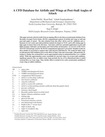
A CFD Database for Airfoils and Wings at Post-Stall Angles ofAttackJustin Petrilli, Ryan Paul,† Ashok Gopalarathnam,‡Department of Mechanical and Aerospace EngineeringNorth Carolina State University, Raleigh, NC 27695-7910andNeal T. Frink§NASA Langley Research Center, Hampton, Virginia, 23681This paper presents selected results from an ongoing effort to develop an aerodynamic database fromReynolds-Averaged Navier-Stokes (RANS) computational analysis of airfoils and wings at stall andpost-stall angles of attack. The data obtained from this effort will be used for validation and refinement of a low-order post-stall prediction method developed at NCSU, and to fill existing gaps inhigh angle of attack data in the literature. Such data could have potential applications in post-stallflight dynamics, helicopter aerodynamics and wind turbine aerodynamics. An overview of the NASATetrUSS CFD package used for the RANS computational approach is presented. Detailed results forthree airfoils are presented to compare their stall and post-stall behavior. The results for finite wingsat stall and post-stall conditions focus on the effects of taper-ratio and sweep angle, with particular attention to whether the sectional flows can be approximated using two-dimensional flow over a stalledairfoil. While this approximation seems reasonable for unswept wings even at post-stall conditions,significant spanwise flow on stalled swept wings preclude the use of two-dimensional data to modelsectional flows on swept wings. Thus, further effort is needed in low-order aerodynamic modeling ofswept wings at stalled conditions.NomenclatureAR aspect ratioa VGRID stretching/growth factorb VGRID stretching/growth factorCFD computational fluid dynamicsCd airfoil or section drag coefficientCf skin friction coefficientCL wing lift coefficientCl airfoil or section lift coefficientCm airfoil or section pitching moment coefficient about the quarter-chordCp pressure coefficientcre f reference chord lengthRe Reynolds number based on airfoil chordSA Spalart-Allmaras turbulence modelTE trailing edge t physical time stepU Freestream reference velocityy non-dimensional wall distance zi height of the ith viscous layerα angle of attack, degΛ angle of sweepback, degλ taper ratio GraduateResearch Assistant, Box 7910, jlpetril@ncsu.edu. Student Member, AIAAResearch Assistant, Box 7910, rcpaul@ncsu.edu. Student Member, AIAA‡ Associate Professor, Box 7910, ashok g@ncsu.edu, (919) 515-5669. Associate Fellow, AIAA§ Aerospace Engineer, Configuration Aerodynamics Branch, MS499. Associate Fellow, AIAA† Graduate
I. IntroductionAirfoil lift and moment data in the low angle of attack regime is readily available from a multitude of sources- fromAbbott and von Doenhoff [1] and those from the University of Stuttgart [2] and University of Illinois at UrbanaChampaign [3,4,5], to modern computational approaches designed to predict sectional aerodynamic characteristicsbased on arbitrary input geometry, such as XFOIL [6]. For many applications, data in this linear regime is sufficient.However, fields such as wind turbine aerodynamics, helicopter aerodynamics and post-stall flight dynamics of fixedwing aircraft require data to extend beyond aerodynamic stall. Efforts have been made in the wind turbine communityand the helicopter aerodynamics community to extend airfoil data into the post-stall regime. In both wind turbine andhelicopter aerodynamics, local blade sections close to the root of the rotor may experience very high angles of attack.Models for airfoil force and moment coefficients at high angle of attack conditions have been developed experimentally[7,8], which has led to researchers proposing empirical models based on flat plate theory [9]. The empirical modelsdeveloped from experiment require that both the maximum Cl and the corresponding α stall at which this lift coefficientoccurs be known reliably before theoretical flat plate data may be fitted to extend the data well into post-stall.Very little data exists in the literature covering the stall behavior of finite wings, especially that which extendsdeep into post-stall. Published work in post-stall wing aerodynamics often covers general stall behavior, dependenton factors such as planform, without providing detailed force and moment data beyond initial stall [10]. Some studiespropose empirical methods based on theory to extend existing force and moment coefficient data-sets deep into poststall taking into account 3D effects with some correction for aspect ratio [8]. An interesting, purely experimental study,that covers the stall of both a 2D airfoil section and 3D wings of various aspect ratios was performed by Ostowari andNaik in 1985 [11]. The study presented consistent lift coefficient versus angle of attack data for various NACA 44XXseries airfoils and 3D rectangular wings with a range of aspect ratios having the same airfoils as cross sections.A database of post-stall airfoil and wing data, with a similar scope to the Ostowari and Naik study, was desiredpartly to address this dearth of data in the literature, but primarily to support a local effort within the Applied Aerodynamics Group at North Carolina State University. The ongoing effort involves developing a low-order model ofpost-stall aerodynamics for finite wings via use of existing linear low-order methods (VLM, Weissinger or LLT) corrected for nonlinear sectional airfoil behavior. Corrections are accomplished via a decambering approach used tomimic the nonlinear aerodynamics caused by flow separation. Details of the development of the low-order methodmay be found in Ref. [12], with the current status pertaining to its use in real-time simulation of aircraft flight dynamics described in Ref. [13]. In addition to geometry information, the low-order post-stall model requires sectional 2Dairfoil data as input for each of the control points. This sectional input data (Cl α, Cd α, and Cm α curves) definesthe convergence criteria for the low-order post-stall calculation for finite wings. Outputs include the total aerodynamicforce and moment coefficients and spanwise distributions of these coefficients.Figure 1 describes the relationship between the low-order method and the higher order Computational Fluid Dynamics (CFD) effort, and how the results from the latter are to be used for initial validation and further refinement ofthe former. Two dimensional CFD is performed on airfoil sections, and the outputs are used as inputs to the low-ordermethod. The 3D geometries utilizing the same 2D cross section are run in both CFD and the low-order method.Theresults are then compared on the basis of total force/moments and spanwise force/moment distributions. CFD solutions and accompanying flow visualizations allow for further development and refinement of the low-order method.Comparisons between the low-order method and CFD are beyond the scope of this paper. This paper aims to discussthe methodology used in generating CFD solutions of airfoils and wings in post-stall angles of attack and to presentthe results in this regime as dependent on geometry and flow conditions.This paper begins by describing the CFD software package that was chosen to generate consistent flow solutionsfor airfoils and wings. The methodology developed to effectively use the CFD package is presented next - fromgenerating usable geometry, creating a suitable grid over the computational domain, running the flow-solver, checkingsolution convergence, and post-processing to extract desired quantities from the outputs. The 2D and 3D results arepresented which show effects from geometry, including wing sweep, and flow parameters. Selected results are shownin more detail using flow visualization and/or spanwise local lift coefficient distributions.2 of 18American Institute of Aeronautics and Astronautics
Figure 1: Approach for using CFD for initial validation and further refinement of the low-order method. Blue emphasizes that a consistent grid spacing is used with the 2D and 3D CFD discretizations.II. Background: NASA Tetrahedral Unstructured Software SystemThe NASA Tetrahedral Unstructured Software System (TetrUSS) [14] is a package of loosely integrated software,developed to allow rapid aerodynamic analysis from simple to complex problems. The system has its origins in 1990 atthe NASA Langley Research Center and has won the NASA Software of the Year Award twice. TetrUSS has been usedon high priority NASA programs such as Constellation and the new Space Launch System for aerodynamic databasegeneration along with work in the Aviation Safety Program. The component software packages are assembled suchthat a user follows a systematic process during each application of TetrUSS. There are software packages for preparinggeometries for grid generation (GridTool), generating unstructured surface and volume grids (VGRID) and calculatingflow solutions (USM3D). Post-processing the solutions with TetrUSS can be done using the included SimpleViewsoftware or by easily converting for use with other commercial packages (eg Tecplot, EnSight etc.).For preparing geometries for grid generation, GridTool is used to generate the necessary VGRID [15] input files.GridTool can read Non-uniform Rational B-Spline (NURBS) curves and surfaces through an Initial Graphics ExchangeSpecification (IGES) file, as well as PLOT3D point cloud surface definitions. The geometric surfaces are then definedby way of surface patch construction. Each patch has a specified boundary condition such as a viscous or inviscidsurface and a family definition for users to group related patches together. Grid spacing parameters are also definedand controlled within GridTool. Sources are placed in three dimensional space by a user in order to control the sizeand growth rates of the tetrahedral cells. Numerous classes of sources are available to control the grid topography.Nodal sources and line sources are typically used in most cases, while volume sources are available for use in specificcases requiring control over a large volume of the domain. Other parameters defined in GridTool are the viscous layerspacing parameters and the maximum and minimum tetrahedral sizes.VGRID is the unstructured grid generation tool used in the TetrUSS Package. Viscous layer generation is accomplished via the Advancing Layers Method (ALM) [16]. Tetrahedral cells are generated in an orderly manner,“marching” nodes away from the surface. The size and growth of these cells is controlled by Equation 1.3 of 18American Institute of Aeronautics and Astronautics
hii zi 1 z1 1 a(1 b)i(1)In this equation, the height of the ith layer is determined by an initial spacing parameter, z1 , and two stretching/growthfactors a and b. Once the height of the ith layer reaches the size of the background sources specified by the user inGridTool, no more cells are formed and viscous layer generation is complete. After the viscous layers are generated,VGRID then utilizes the Advancing Front Method (AFM) [17] for the generation of the inviscid portion of the volumegrid. VGRID can not always close the grid completely. When this occurs, a slower but more robust auxiliary codecalled POSTGRID is used to complete the formation of the remaining tetrahedral cells.The flow solver at the core of the TetrUSS package is USM3D [18]. USM3D is a parallelized, tetrahedral cellcentered, finite volume Reynolds Averaged Navier-Stokes (RANS) flow solver. It computes the finite volume solutionat the centroid of each tetrahedral cell and utilizes several upwind schemes to compute inviscid flux quantities acrosstetrahedral faces. USM3D has numerous turbulence models implemented for use; the Spalart-Allmaras (SA) oneequation model and Menter Shear Stress Transport (SST) two equation model were used in this study. Some additionalcapabilities that USM3D has implemented are dynamic grid motion and overset grids.III. Methodology: Developing the Aerodynamic DatabaseThe aerodynamic database is desired to have high fidelity flow solutions for a wide variety of 2D airfoils and 3Dgeometries. Flow solutions would include a large range of angles of attack to encompass pre-stall, stall and post-stallflow regimes. The data gained from these simulations will be vital in assisting the further development and validationof the low-order method mentioned in the introduction as well as to fill gaps in the currently available high angle ofattack aerodynamic data for arbitrary geometries. An efficient process to go from a geometry to a converged flowsolution was developed and is discussed in the following sub-sections.A.Geometry GenerationTraditional Computer Aided Design (CAD) software would be more than adequate for the creation of the desiredgeometries, however these tools are not geared specifically towards the modeling of wings and airfoils. Understandingthis, the recently released parametric modeling tool, Open Vehicle Sketch Pad (OpenVSP) [19], was chosen as thegeometry generation tool. A flow chart showing the process of geometry generation can be seen in Figure 2. OpenVSPis a modeling package developed and released by NASA Langley Research Center in Hampton, Virginia. The uniqueconcept that OpenVSP provides is that it allows a user to drag and drop generic aircraft components (such as a wing)into the modeling area, and directly manipulate familiar geometric parameters. Consequently, it is simple to insert awing, change its root chord, tip chord, span, etc. and view the resulting geometry in real time. Aerodynamic referencequantities can also be automatically calculated for the user. Airfoils cross section generation is also simplified. Auser can select any 4 or 5 digit series NACA airfoil or load in a formatted airfoil coordinate file for use on any liftingsurface.The 3D wing and corresponding airfoil for each case to be analyzed were generated in OpenVSP. In order to readthe geometry into GridTool, the file must be in the IGES format. Vehicle Sketch Pad does not output IGES files,thus each geometry must be exported as a Rhino3D formatted file. The Rhinoceros NURBS modeling package wasused to convert the geometry into the necessary IGES file as well as make small modifications to the geometry. Somegrid generation failures were encountered due to how OpenVSP closes the trailing edge of the wing/airfoil geometries(it always forces a sharp trailing edge). In some cases the sharpness had to be removed to ensure successful gridgeneration.4 of 18American Institute of Aeronautics and Astronautics
Figure 2: Process of geometry generation to grid generationB.Grid GenerationGrid generation parameters were generalized such that, between different geometries, parameters such as source placement and viscous spacing had minimal required changes. This meant that from initial geometry generation to a completed grid would require only a matter of hours. Establishing this commonality and routine for grid generation enabledthe generation of adequate grids for many configurations in a short time span. An example placement of sources fora simple tapered wing is shown in Figure 3. A series of line sources are utilized, in the spanwise direction of eachwing at differing chord-wise locations. Anisotropic stretching [20] as high as 10:1 was used near the root of the wing,transitioning to isotropic cells near the wing tips. For viscous tetrahedral layer generation, the height of the first layer( z1 ) is Reynolds number dependent. A viscous layers spacing tool called USGUTIL, was used to determine theheight of the initial viscous layer. In order to have adequate number of cells in the viscous layers, the y of the firstnode was set to be 3, this would ensure that the y of the first cell center would be less than 1 (approx. 0.75) as isrequired for a fully viscous Navier-Stokes solution. The values used for the grid growth parameters (a and b) in Eq.1 were 0.15 and 0.02 respectively [20]. A grid sensitivity study was performed on a rectangular wing with aspectratio of 12 to determine adequate grid sizing. It was found that a grid sizing of 5–9 million tetrahedral cells showedchanges in C L,max of approximately 0.02 between the grids. This method of grid generation was applied to all 3D winggeometries with the typical grids averaging between 9–12 million tetrahedral cells.For airfoil calculations, a quasi 2D grid was generated on a constant-chord, short-span wing, between two reflectionplane boundary condition patches. Figure 4 shows a completed grid for an NACA 0012 airfoil. A general goal wasset to maintain very similar grid density between the 3D wing grids and the airfoil grids. This is necessary becausethe airfoil results were being used as input data into the low-order method discussed in the introduction while the 3Dwing results from USM3D were being used to assess the accuracy of the low-order method (Figure 1). Therefore aseparate grid sensitivity study was not performed specifically for airfoils. Typical airfoil grids were on the order of300,000 tetrahedral cells and were generated using a nearly identical source placement as the 3D wing.C.Flow Solution GenerationAll solutions with the USM3D solver were computed with time-accurate Reynolds-Averaged Navier-Stokes (RANS).The limitations of RANS for modeling massively separated flows are well known. The more preferred Detached EddySimulation (DES) modeling will provide better physical representation of 3D separated flow, but with an order-ofmagnitude more expense. Since this investigation requires generation of many flow solutions, the initial focus is todetermine if time-accurate RANS can provide sufficient engineering accuracy for capturing the salient aerodynamiccharacteristics of wings at stall and post-stall conditions. Furthermore, a consistent modeling is desired between the2D airfoils and 3D wings.All computations were advanced at a characteristic time step of t t · U /cre f 0.02 using a second order time-accurate scheme with three-point backward differencing and physical time stepping. The number of subiterations for each time step was set to between 10 and 15 to ensure adequate sub-iteration convergence. The Spalart-5 of 18American Institute of Aeronautics and Astronautics
Figure 4: Screen capture of airfoil grid.Figure 3: Screen capture of GridTool source placementon a tapered wing.Allmaras (SA) [21] one equation turbulence model was used almost exclusively, however some simulations wereperformed with the two equation SST turbulence model to understand the difference in final solution quantities. Thesolver was run on both a NASA Langley computer cluster and the North Carolina State University High PerformanceComputing (NCSU HPC) cluster. Making use of USM3D’s parallel computation capabilities, each grid was partitioned into 28-64 equal zones which could be loaded onto 28–64 individual processors, reducing calculation timessignificantly. To further increase productivity, a series of Unix scripts were developed to generate the required inputfiles for job submission and minor post-processing of completed jobs.D.Solution ConvergenceConvergence of the solutions was monitored by generating convergence plots such as that seen in the Figure 5. Unixscripts were used to compile all of the convergence information contained in the USM3D output files into a Tecplotformat. Each plot showed the logarithm of the residual over each iteration and the changes in the aerodynamic coefficients. The criteria for a fully converged solution was for each plot to show a leveling off of the quantities underconsideration. These plots allowed for rapid determination of whether any given solution had reached a convergedstate (Figure 5a) or if the solution had attained an unsteady solution shown by oscillatory convergence (Figure n34000.54x 10a) Smooth convergence, α 30deg.11.5iteration22.534x 10b) Oscillatory convergence, α 48deg.Figure 5: Typical USM3D convergence of lift coefficient for an airfoil. NACA 4415, USM3D/SA, RE 3 million,M 0.2.6 of 18American Institute of Aeronautics and Astronautics
E.Post-ProcessingAfter solution convergence was verified, the data is processed so that total forces and moments, the spanwise distribution of forces and moments, and flow visualization may be studied. As was previously mentioned, in some casesan oscillatory solution develops rather than single steady-state values for the forces and moments. This has only beenobserved for 2D airfoil solutions at very high angles of attack. To handle such cases, a method had to be developed inorder to address these oscillations.1.Forces and moments acting on the entire wing/configurationThe first outputs of interest are the total force and moment coefficients acting on a wing/configuration. Ascript was used to extract the body-axis force and moment coefficients [C X CY CZ C Mx C My C Mz ], defined parallel and perpendicular to the body coordinate system,and stability-axis coefficients [C L C D ], defined paralleland perpendicular to the free-stream velocity. Figure 6shows an example of lift coefficient results for a 2D airfoil and a 3D wing which used the same airfoil crosssection.1.8AirfoilWing1.61.4Cl , CL1.210.80.62.Span-wise distribution of forces on a surface0.4The other output of interest is the span-wise distribution0.2010203040of force coefficients, particularly the span-wise lift coefα(deg)ficient. The PREDISC utility [22], was used for extracting this information. PREDISC simultaneously loadsthe grid files containing the surface grid and a convertedTetrUSS solution file containing only surface data. Data Figure 6: Comparison of lift coefficients for 2D airfoilextraction planes can be arbitrarily defined (see Figure (NACA 4415) and AR 12 rectangular wing at RE 37) and PREDISC will output surface pressure and skin million.friction coefficients, C p and C f respectively, along thesurface discretized according to a fine mesh of x/c, y/c locations. The surface pressure and skin friction coefficientsare integrated to approximate body-axis force coefficients. An example lift coefficient distribution obtained by integrating the C p and C f values at each extraction plane is shown in Figure 7.1.8Section Cl1.61.41.210.80246Spanwise distance (y)8Figure 7: Screen shot of PREDISC code (left) showing defined data extraction planes and a plot of the extractedspanwise Cl distribution (right) on a rectangular wing AR 12.7 of 18American Institute of Aeronautics and Astronautics
IV.ResultsThe results shown in this section represent the current level of development of the CFD database. The results fromanalysis of 2D airfoil CFD solutions for cambered, symmetric and thin airfoils will be presented along with 3D wingsolutions with rectangular, tapered and swept planforms.A.2D Airfoil Resultsy/cThree different airfoils have been studied and added to the CFD aerodynamic database to date. Additional airfoils will be added as neededNACA 0012for further development of the database and as required for validationNACA 4415of the low-order post-stall method discussed previously. The airfoils0.4NACA 63006chosen exhibit different stall and post-stall behavior and offer insight0.3on how certain airfoil geometries will tend to behave at high angles0.2of attack. Results for a symmetric airfoil (NACA 0012), a cambered0.1airfoil (NACA 4415) and a very thin airfoil (NACA 63006) are shown0in this section. The geometries of the airfoils are shown in Figure 8. 0.1One interesting phenomenon that was encountered while devel 0.2oping the airfoil database, was the tendency for the airfoil solutionsto exhibit oscillatory behavior in the force and moment convergence00.20.40.60.81histories at angles of attack of approximately 40 degrees and above.x/cThe cause of these oscillations was determined using flow visualization which revealed periodic vortex shedding from the upper surfaceof the airfoil. A process to average the oscillatory behavior and de- Figure 8: Comparision of airfoil geometry fortermine peak to peak amplitudes was established. A post-processing the three cases studied.MATLAB script was developed to read all of the force and momenthistory files for an airfoil and detect the oscillatory behavior. For any angle of attack that displayed this behavior, thescript identified two complete cycles at the end of the convergence history and determined the mean value along withthe peak to peak amplitude. The plots in Figure 9 illustrate the approach used for the processing of the raw CFD datawith this code.raw cfd dataCl42000.511.52iteration2 complete cycles identified2.534x 10Cl1.51Convergence history data2 complete cycles0.5Average of 2 complete cycles022.22.42.62.8iteration34x 10Figure 9: Illustration of approach used for averaging oscillator airfoil CFD convergence history.8 of 18American Institute of Aeronautics and Astronautics
1.Reynolds Number Effects Through Post-StallThe general effects of Reynolds number on the aerodynamic quantities, specifically Cl,max , are known and have beenobserved with the current work as well. However, it is important to extend this to the post-stall region. Figure 10 showsa comparison of the lift curves for the NACA 4415 airfoil at three different Reynolds numbers (3, 6 and 10 million).The increased maximum lift coefficient with increased Reynolds number is expected. In the post stall region betweenangle of attack of 40 and 70 degrees, an additional effect of the Reynolds number is seen. The region falls directlywhere the oscillatory solutions develop; the values shown in Figure 10 are the averaged values from any oscillatingdata. After this recovery region, the solutions tend to follow a similar path out to 90 degrees.2.Sharp vs. Blunt Trailing Edge GeometriesIt has been noted by Hoerner [23], that the trailing edge shape of an airfoil has a distinguishable effect on the Cl vs.α curve. When comparing an airfoil with a sharp trailing edge with the same airfoil but with a blunt trailing edge, itis found the the maximum lift coefficient is seen to be higher for the blunt trailing edge airfoil. The plot in Figure11 displays results for an NACA 4415 airfoil with both a sharp and blunt trailing edge at a Reynolds number of 3million. The blunt TE geometry was generated by removing the final one percent of the chord of the sharp trailingedge geometry, thus no other alterations to the geometry are present. The expected trend is seen with the blunt trailingedge case having a higher maximum lift coefficient. It is interesting to see that this effect seems to continue all theway past stall and through to approximately α 70 degrees, after which the lift curves coincide. The flow mechanismthat allows for this all the way through post stall is not readily apparent from the CFD at this time, but warrants furtherinvestigation.NACA 4415 RE3m Sharp TENACA 4415 RE3m22NACA 4415 RE6mNACA 4415 RE3m Blunt TENACA 4415 �Figure 10: Effect of Reynolds number on lift coefficient for an NACA 4415 airfoil. USM3D/SA, M 0.2.3.40Figure 11: Effects of trailing-edge sharpness for anNACA 4415 airfoil. USM3D/SA, Re 3 million, M 0.2.Comparison of Post-Stall Characteristics of Three Airfoil GeometriesAirfoils that exhibit different characteristics in terms of maximum lift coefficient and stall behavior were analyzedfor addition to the post-stall database. In Figure 12, lift curves for three airfoils are shown from 0 to 90 degreesangle of attack. A cambered airfoil (NACA 4415), a symmetric airfoil (NACA 0012) and a very thin airfoil (NACA63006) are compared in the figure. The NACA 4415 and NACA 0012 both exhibit trailing edge stall behavior. Thatis, flow separation begins at the trailing edge and progresses towards the leading edge as the angle of attack increases.This can be seen in the lift curves as both the airfoils have a relatively “gentle” stall. It is interesting to note thatalthough the NACA 4415 airfoil has a higher Cl,max as compared to the NACA 0012, the two airfoils have very similarmaximum recovery lift coefficients at approximately 50 degrees angle of attack. The NACA 63006 produced a much9 of 18American Institute of Aeronautics and Astronautics
more unusual lift curve. This airfoil is categorized as having “thin airfoil” stall characteristics. Due to the presence ofa severe adverse pressure gradient around the leading edge at even low angles of attack, the flow over the upper surfacecompletely separates. This sudden onset of flow separation can been seen by the sudden leveling of the lift coefficientat around 10 degrees. After this initial “stall”, the airfoil recovers past the initial stall lift coefficient and reaches nearlythe same maximum recovery Cl at α 50 degrees as the NACA 4415 and NACA 0012. The differences seen betweenthese three airfoils in the 40 to 60 degree range can mainly be attributed to thickness, camber and leading-edge radiuseffects.An enlarged plot of the NACA63006 in the region of incipient stall is shown in Figure 13 with comparison toexperimental data obtained from Abbott and von Doenhoff [1] and also noted by Hoerner [23]. It should be notedthat since the CFD solutions were fully turbulent (no transition model was used) no evidence or effects of a laminarseparation bubble near the leading edge were modeled, a phenomenon noted by Leishman and in other studies ofsimilar airfoils [24].1.80.9NACA 4415NACA 0012NACA .20.1NACA 63006 ExperimentalNACA 63006 CFD0020406080010002αFigure 12: Comparison of Cl vs. α for three airfoiltypes. USM3D/SA, Re 3 million, M 0.246α81012Figure 13: Comparison of Cl vs. α from CFD andexperiment for the NACA 63006 thin airfoil.Figures 14 and 15 show Mach number contour plots along with surface C p distributions for the NACA 4415 andNACA 63006 airfoils at diff
the methodology used in generating CFD solutions of airfoils and wings in post-stall angles of attack and to present the results in this regime as dependent on geometry and flow co nditions. This paper begins by describing the CFD software package that was chosen to generate consistent flow solutions for airfoils and wings.