WIXLIB

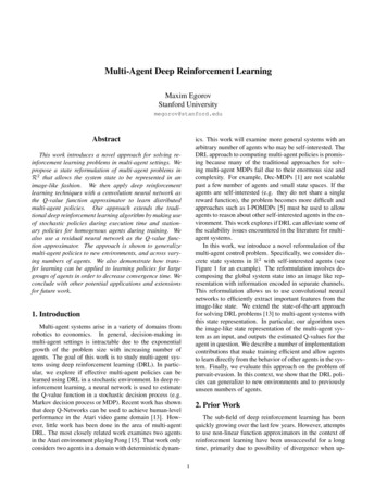
also called neurons. An ANN is called a feedforward ANN if there are nofeedback connections of the output of the ANN being sent to itself. Each neuronis a linear function of some inputs, fed into a nonlinear function, called activationfunction. If the input of a neuron is a vector x, the output of the neuron gi canbe written asgi K(ωi x bi ).(2.1)Here K is the non-linear activation function, ω is a vector consisting of someweights and bi is a bias. Note that x (x1 , ., xN ) is an N dimensional vector,where N is the number of inputs into gi . The output of a neuron is typicallyused as one of many inputs to the next layer of neurons. A deep ANN hasmultiple neurons that take the same inputs, then all of those neurons’ outputsare combined to a new vector that is input to the next vector and so on. Anentire layer can be written in terms of matrix multiplications asg K(W x b),(2.2)where W is the matrix W (ω1 , ., ωN ) and the bias vector b (b1 , ., bN ) and K is the vector valued activation function.Layers that are not the the first or the last layer in a ANN are called hiddenlayers. The more layers a ANN has, the deeper it is said to be. An illustrationof a simple network with one hidden layer and a single output neuron can beseen in Figure igure 2.1: A basic feedforward ANN which consists of an input layer, a hiddenlayer and an output layer.A ANN is then trained to approximate a given function by updating its parameters, the weights and the biases. Usually the parameters are denoted by θ andthe entire function that is the ANN can be written as y f (x; θ), where y isthe output of the ANN, x is the input and θ are all the variable parameters. [6,Chapter 6]6

2.3.1Activation FunctionsThe non-linear functions called activation functions, such as K in Equation 2.1,are typically fixed non-linear functions that are used to make the ANN able toapproximate non-linear functions. If the non-linear activation functions weren’tused, the output of the ANN would still be a linear function of the inputs x[6, Chapter 6]. In deep learning, there are a few commonly used functions thathave become standard as activation functions.The rectifying linear unit, or ReLU is a function that is defined asReLU(x) max(0, x).(2.3)The ReLU function is continuous and piece-wise linear with just one point withdiscontinuities in the derivatives. Since the function is almost linear many goodproperties of linear functions are preserved in terms of ease of optimization withgradient based methods. ReLU functions can however sometimes be problematic due to the gradients being zero if the input to the ReLU function is lessthan zero. This can for instance be solved by using leaky ReLU functions, wherethere is a small slope for inputs with values less than zero [6, Chapter 6].Another common activation function is the logistic sigmoid function,σ(x) 1.1 e x(2.4)The logistic sigmoid function σ(x) outputs values in the range (0, 1) and canbe interpreted as the probability P (x 1) from a Bernoulli distribution. [6,Chapter 3] This is also commonly used as the last layer in classification problems with just a single class of interest.Another common activation function is the hyperbolic tangent, tanh. It is verysimilar to the sigmoid function, but it outputs values in the range ( 1, 1). Infact the hyperbolic tangent and the logistic sigmoid function are related,tanh (x) 2σ(2x) 1.(2.5)The tanh function is centered around zero and is close to linear around 0, whichmakes training ANNs easier with the hyperbolic tangent function compared tothe sigmoid. However, both the hyperbolic tangent and the sigmoid functionhave to a large extent been replaced by the ReLU function and variants of itas the standard for hidden units in practice. Both the hyperbolic tangent andthe sigmoid function are however commonly used for output layers. Activationfunctions is still an active area of research and the ones presented here arecommonly used, but there are many other options that have similar performance[6, Chapter 6].7

2.3.2Cost FunctionsTo train a ANN, cost functions are usually minimized. In supervised learning, where we have labeled data to learn from, the cost functions are morestraightforward than for instance in reinforcement learning that we will discussin section 2.4.The two main problems of supervised learning are regression and classification.In regression one wants to predict a numerical value whereas in classification thegoal is to predict which class something belongs to given some inputs. Differentloss functions are common for regression and classification. Most of them arehowever derived from the same principle, the one of Maximum Likelihood.Maximum likelihood involves finding some parameters θM L such thatθM L arg max pmodel (X; θ).(2.6)θHere X {x1 , ., xn } is the set of input data that comes from the distributionthat we want to approximate with pmodel , and pmodel is some chosen class ofprobability density functions parameterized by θ. This can be written as aproduct over each input data point,θM L arg maxθnYpmodel (xi ; θ).(2.7)i 1Maximizing this is equivalent to maximizing the logarithm of the product, whichis more commonly done since it has better numerical properties,θM L arg maxθnXlog pmodel (xi ; θ).(2.8)i 1If we divide by the number of samples n we can getθM L arg max Ex ptrue log pmodel (x; θ).(2.9)In the supervised learning setting, we have both known target values or labelsY {y1 , ., yn } and input data X {x1 , ., xn }, so we want to find θM L suchthatθM L arg max pmodel (Y X; θ).(2.10)θIf the samples are independent and identically distributed we can get θ as8

θM L arg maxθnXlog pmodel (yi xi ; θ),(2.11)i 1orθM L arg max Ex ptrue log pmodel (y x; θ).(2.12)[6, Chapter 5]The Mean Squared Error, or MSE can be derived by assuming thatpmodel (y x, θ) N (y f (x, θ), I).(2.13)Maximizing this is equivalent to minimizing the MSE,nJM SE (θ) 1X yi f (xi , θ) 2 ,n i 1(2.14)which is shown in [6, Chapter 5].A cost function related to the MSE is the Huber loss. In Tensorflow it is definedas(JHuber (θ) 1 22y1 22d d( y d)if x dif y d.(2.15)Here d is a design parameter that determines where the loss function changesfrom quadratic to linear and y is the error between the predicted value and thereal value [8].2.3.3Back-propagationWhen training a ANN to approximate a function, gradient based optimizationis commonly used. To compute the gradient of a (loss) function f (x; θ) withrespect to the parameters θ an algorithm called back-propagation is commonlyused. It back-propagates from the objective function to gradients of the differentweights and biases in the ANN to compute the gradient of the objective function with respect to all the parameters. If we have a function f (x; θ), we usuallywant to compute the gradient θ f (x; θ) of f with respect to θ to improve theANN with respect to this function f , that is some measure of performance. Itcan be a cost function in a supervised learning setting but could also be otherfunctions like a reward function in the reinforcement learning setting that will9

be introduced in a later section.The backprop algorithm uses the chain rule from calculus for each layer of theANN at a time. If we have z f (g(x)) and y g(x), all functions and variablesvector valued, we can compute the gradient of z with respect to x like z z ( y ) y z, x(2.16) ywhere ( x) is the Jacobi matrix of y(x). What the backprop algorithm does isto just compute the gradient like this for each layer in the ANN step by stepfor each layer. The algorithm avoids computing the same expressions multipletimes which makes it numerically efficient. [6, Chapter 6]2.3.4Gradient based optimization for deep learningThe ANN weights and biases are updated to optimize some objective functionwith gradient based optimization, using the gradients computed with the backprop algorithm.The classic algorithm for optimizing the parameters in a ANN is called GradientDescent. Let L(x; θ) be an objective function that we want to minimize, wherex is the input to the ANN and θ are the trainable parameters of the ANN. Thenmoving in the opposite direction of the gradient of L with respect to θ we movethe parameters in a direction that makes the objective function smaller, which iswhat we want. However, usually x are random samples and the true gradient isthe expected value of the gradient with respect to the random samples actuallyused. Thus when computing the gradient of the loss function as a function ofsome samples x, we are computing an unbiased noisy estimate of the gradient.This is referred to as Stochastic Gradient Descent, or SGD. Stochastic GradientDescent as presented in [6, Chapter 8] can be seen in Algorithm 1.Algorithm 1 Stochastic Gradient DescentRequire: Learning rate schedule 1 , 2 , .Require: Initial parameters θk 1while Stopping criterion not met doSample a minibatch of m examples from the training set {x(1) , ., x(m) }with corresponding targets y (i)P1(i)(i)Compute gradient estimate: ĝ mi L(f (x ; θ), y )Apply update: θ θ k ĝk k 1end while10

Note that we are using a learning rate schedule in Algorithm 1. That is, whentaking steps in the direction of the gradient we are using some schedule for howlong along the gradient direction we should go in our updates. Another alternative to this is to do a Line Search, that is to find the step size that minimizesthe function along this direction for each step. To guarantee convergence whenusing a learning rate schedule with learning rate , the condition that X k ,k 1 X 2k (2.17)(2.18)k 1is a sufficient condition [6, Chapter 8].One problem with SGD is that it can easily get stuck in local minima, since whenthe gradient is 0, we will not move any more. One popular way of dealing withthis is to use the Adam algorithm for optimization. Adam is an algorithm thatuses adaptive learning rate and momentum. Adaptive learning rate means thatthe learning rate is determined by the algorithm itself, using some chosen baselearning rate. Momentum is a way of making the algorithm try to avoid badlocal minimums by keeping track of a moving, exponentially decaying, averageof the past gradients and moving in that direction instead of only the currentgradients direction. Adam keeps track of two different orders of momentum andcorrects the biases that comes from the initialization of the momentum. TheAdam algorithm as presented in [6, Chapter 8] can be seen in Algorithm 2.2.3.5Batch NormalizationBatch Normalization is a recent method in deep learning used to be able to trainnetworks faster and use higher learning rates with decreased risk of divergence.It does so by making the normalization a part of the model architecture, fixingthe mean and variances of the inputs to a layer by a normalization step. Thismakes the risk of the inputs to the activation functions getting in a range wherethe gradient vanishes smaller and allows for the use of higher learning rates. [9]2.4Reinforcement LearningA Markov Decision Process, or MDP, is the mathematical framework aroundwhich RL is built. There is a learner and decision maker, called the agent thatinteracts with an environment. There is a set of actions A, a set of states S anda set of observations O.Given a state S, we have all necessary information about the state of the systemwith just the latest state. This is called the Markov property. The observations11

Algorithm 2 AdamRequire: Step size (Suggested default: 0.001)Require: Exponential decay rates for moment estimates ρ1 and ρ2 in [0, 1).(Suggested defaults: 0.9 and 0.999 respectively)Require: Small constant δ used for numerical stabilization. (Suggested default:10 8 )Require: Initial parameters θInitialize 1st and 2nd moment variables s 0, r 0Initialize time step t 0while Stopping criterion not met doSample a minibatch of m examples from the training set {x(1) , ., x(m) }with corresponding targets Py (i)1(i)(i)Compute gradient: ĝ mi L(f (x ; θ), y )t t 1Update biased first moment estimate: s ρ1 s (1 ρ1 )gUpdate biased second moment estimate: r ρ2 r (1 ρ2 )g · gsCorrect bias in first moment: ŝ 1 ρt1rCorrect bias in second moment: r̂ 1 ρt2ŝCompute update: θ r̂ δ(operations applied element-wise)Apply update: θ θ θend whileare observations of the underlying state, but they might not convey all information that is in a single state. If the observations don’t convey all informationabout the state the MDP is said to be a Partially Observed Markov DecisionProcess, or POMDP and then the system does not satisfy the Markov property.The agent performs actions ai A based on an observation Oi O. After performing an action at time t the agent receives a real valued reward, Rt R andthe state changes according to the MDP. This is illustrated in Figure 2.2. Herethe word state is used to describe the observations, which in ideal circumstancesare complete representations of the state.The goal of the agent is to maximize the expected value of the return. Thereturn at time step t, here denoted Gt is a function of the current and futurerewards and can be defined as follows:Gt Rt γRt 1 γ 2 Rt 2 γ 3 Rt 3 . Rt γGt 1 .(2.19)Here γ [0, 1] is called the discount factor. The smaller the discount factor,the more emphasis is put on short term rewards. If γ 1 the return of aninfinite sequence is finite as long as the rewards are bounded. Examples of infinite sequence would be a robot that walks or a car that should drive on a roadand similar scenarios. If the agent does tasks in episodes the task is said to be12

AgentNew state st 1Reward rt 1Action atEnvironmentFigure 2.2: A sketch of an agent interacting with an environment. The agentreceives a state and reward from the environment, the agent outputs an actionand the environment updates according to the underlying MDP.episodic. That is, the task finishes after some episodes when the environmentreaches a state called the terminal state.If we don’t know how the transitions between states given some actions are andwant to maximize the return we are dealing with the problem of model free RL.Formally the goal of reinforcement learning is to find a policy π(s), sometimeswritten as π(a s), that is a mapping from the observations to different actionsor probabilities of different actions to be selected such that it maximizes theexpected return [10].Given a state s, action a and a policy π(s) there exists a State Value functionvπ (s) and a state-action value function qπ (s, a) associated to the policy π. Thesefunctions tell us how good it is to be in a state or how good it is to perform anaction in a given state. They are defined as following:vπ (s) Eπ [Gt St s] Eπ [r γGt 1 St s],(2.20)qπ (s) Eπ [Gt St s, At a] Eπ [r γGt 1 St s, At a].(2.21)Note that the value functions tell us the value of a state or state-action pairgiven a specific policy π. These functions can be estimated, for instance onecan use Monte Carlo methods to keep track of the average returns followinga state or a state-action pair. If the state space and/or action space is largethese functions are typically approximated by parameterized functions such asfor instance ANNs and the parameters are updated to fit the observed returnsafter running the policy π.For an MDP there also exists an optimal policy with associated optimal statevalue and state-action value functions. An optimal policy π is a policy suchthat vπ (s) vπ0 (s) for all policies π 0 , and similarly for the state-action valuefunction. [10, Chapter 3]13

2.4.1Exploration vs exploitationA common dilemma in reinforcement learning is the exploration vs exploitationdilemma. Should the agent do what it thinks is the best or should it try newthings in order to potentially find better actions that it doesn’t know aboutyet? In order to find an optimal policy the agent needs to explore, but it shouldalso use the knowledge of what it thinks is good. The problem with this tradeoff is called the exploration vs exploitation dilemma and is an active researchproblem.2.4.2TD-learningIn Temporal Difference learning, or TD-learning, the state-value or state-actionvalue function is updated with approximations and the recursive relationshipsin Equations (2.20) and (2.21). For instance, it is possible to approximate thevalue function with vπ (s) V (s) for a given policy given many updates of theformV (st ) V (st ) α[Gt V (st )],(2.22)here Gt can be approximated with for instanceGt Rt γV (st 1 ).(2.23)When such an approximation is used, that is when the whole discounted rewardGt isn’t used we are dealing with TD-learning. Using the recursive relationshipfrom Equation (2.19) to update the estimated state-value of state-action valuefunction is known as bootstrapping in reinforcement learning contexts. This iscalled the one step return. If we instead of using only the reward for the nextstep and the value function for approximating the value use n different stepslikeGt Rt γRt 1 . γ n 1 Rt n γ n V (st n ).(2.24)This is called the n-step return.2.4.3Q-learningOne common TD-learning algorithm is Q-learning. In Q-learning the optimalstate-action value function, also called the Q-function, is approximated and theactions can then be selected greedily so that the agent takes the action with thelargest state-action value function at each time step. If the approximated stateaction value function is the optimal one, the policy generated by this strategyis also the optimal policy. In Q-learning the approximated optimal state-actionvalue function Q(s, a) is initialized in some way, then actions a are taken and14

Q(s, a) is updated to minimize the Temporal Difference error, or TD-error attime step i,ei yi Q(si , ai ),(2.25)yi Ri γ max Q(s0i , ai ).(2.26)whereawhere s0 is the state following taking action a in state s. Note that the action that maximizes the Q-function is chosen for the Q-value at the next step.Finding the optimal Q-function can be accomplished by iteratively updating theQ-function in the following wayQ(s, a) Q(s, a) α[Rt γ max Q(s0 , a) Q(s, a)].a(2.27)Which will converge to the true optimal Q-function as the number of steps goesto infinity. [10, Chapter 6]2.4.4Policy gradientIt is also possible to learn a policy directly without estimating any value functions. It is done by starting with some rand

in the programming language Python so an interface between existing Matlab code for the model and the reinforcement learning agent must be made with certain added functionality which will be discussed in section 3.2. . Deep Learning is a term used for training deep arti cial neural networks, or ANNs. An ANN is a function approximator .