Transcription
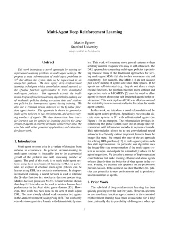
Multi-Agent Deep Reinforcement LearningMaxim EgorovStanford Universitymegorov@stanford.eduAbstractics. This work will examine more general systems with anarbitrary number of agents who may be self-interested. TheDRL approach to computing multi-agent policies is promising because many of the traditional approaches for solving multi-agent MDPs fail due to their enormous size andcomplexity. For example, Dec-MDPs [1] are not scalablepast a few number of agents and small state spaces. If theagents are self-interested (e.g. they do not share a singlereward function), the problem becomes more difficult andapproaches such as I-POMDPs [5] must be used to allowagents to reason about other self-interested agents in the environment. This work explores if DRL can alleviate some ofthe scalability issues encountered in the literature for multiagent systems.In this work, we introduce a novel reformulation of themulti-agent control problem. Specifically, we consider discrete state systems in R2 with self-interested agents (seeFigure 1 for an example). The reformulation involves decomposing the global system state into an image like representation with information encoded in separate channels.This reformulation allows us to use convolutional neuralnetworks to efficiently extract important features from theimage-like state. We extend the state-of-the-art approachfor solving DRL problems [13] to multi-agent systems withthis state representation. In particular, our algorithm usesthe image-like state representation of the multi-agent system as an input, and outputs the estimated Q-values for theagent in question. We describe a number of implementationcontributions that make training efficient and allow agentsto learn directly from the behavior of other agents in the system. Finally, we evaluate this approach on the problem ofpursuit-evasion. In this context, we show that the DRL policies can generalize to new environments and to previouslyunseen numbers of agents.This work introduces a novel approach for solving reinforcement learning problems in multi-agent settings. Wepropose a state reformulation of multi-agent problems inR2 that allows the system state to be represented in animage-like fashion. We then apply deep reinforcementlearning techniques with a convolution neural network asthe Q-value function approximator to learn distributedmulti-agent policies. Our approach extends the traditional deep reinforcement learning algorithm by making useof stochastic policies during execution time and stationary policies for homogenous agents during training. Wealso use a residual neural network as the Q-value function approximator. The approach is shown to generalizemulti-agent policies to new environments, and across varying numbers of agents. We also demonstrate how transfer learning can be applied to learning policies for largegroups of agents in order to decrease convergence time. Weconclude with other potential applications and extensionsfor future work.1. IntroductionMulti-agent systems arise in a variety of domains fromrobotics to economics. In general, decision-making inmulti-agent settings is intractable due to the exponentialgrowth of the problem size with increasing number ofagents. The goal of this work is to study multi-agent systems using deep reinforcement learning (DRL). In particular, we explore if effective multi-agent policies can belearned using DRL in a stochastic environment. In deep reinforcement learning, a neural network is used to estimatethe Q-value function in a stochastic decision process (e.g.Markov decision process or MDP). Recent work has shownthat deep Q-Networks can be used to achieve human-levelperformance in the Atari video game domain [13]. However, little work has been done in the area of multi-agentDRL. The most closely related work examines two agentsin the Atari environment playing Pong [15]. That work onlyconsiders two agents in a domain with deterministic dynam-2. Prior WorkThe sub-field of deep reinforcement learning has beenquickly growing over the last few years. However, attemptsto use non-linear function approximators in the context ofreinforcement learning have been unsuccessful for a longtime, primarily due to possibility of divergence when up1
lowing rule:Q(s0 , a0 ) Q(s, a)). (1)Q(s, a) Q(s, a) α(r γ max0aWhere Q(s, a) denotes the utility of taking action a fromstate s. Q-learning can be directly extended to DRL frameworks by using a neural network function approximatorQ(s, a θ) for the Q-values, where θ are the weights of theneural network that parametrize the Q-values. We updatethe neural network weights by minimizing the loss function:Figure 1. Example instance of a pursuit-evasion game, where thetwo pursuers (red agents) are attempting to catch the two evaders(blue agents). The agents are self interested, i.e. the pursuers andthe evaders have different objectives. The filled in grid points indicate obstacles through which the agents cannot pass.L(s, a θi ) (r γ max Q(s0 , a θi ) Q(s, a θi ))2 . (2)aThe backpropogation algorithm is used to update the network weights at iteration i 1 by performing the computation: θi 1 θi α θ L(θi ). In this work the ADAMupdate rule [7] was used. The use of neural networks a Qvalue function approximators was an open research challenge for a long time. The two insights that significantlyimprove convergence and training rates are the use of experience real dataset and the use of a target Q-network forcomputing the loss. The experience replay dataset contains a fixed number of transition tuples in it that contain(s, a, r, s0 ) where r is the reward obtained by performingaction a from state s, and s0 is the state the agent transitions to after performing that action. The experience tuplesare sampled uniformly from the experience replay datasetin mini batches, and are used to update the network. Theaddition of experience replay helps prevent correlation between training samples, which improves convergence. Theuse of a target network in the loss function calculation helpsconvergence as well. The target network in the loss functionQ(s0 , a θi ) is kept fixed for a certain number of iterations,and is updated periodically.date schemes are not based on bound trajectories [16]. Recent work has demonstrated that using neural networks forapproximating Q-value functions can lead to good resultsin complex domains by using techniques like experience replay, and target networks during updates [13], giving birthto deep reinforcement learning. Deep reinforcement learning has been successfully applied to continuous action control [9], strategic dialogue management [4]and even complex domains such as the game of Go [14]. Also, a number of techniques have been developed to improve the performance of deep reinforcement learning including doubleQ-Learning [17], asynchronous learning [12], and duelingnetworks [19] among others. However, work on extending deep reinforcement learning to multi-agent settings hasbeen limited. The only prior work known to the author involves investigating multi-agent cooperation and competition in Pong using two deep Q-Network controllers [15].This work aims to fill a part of that gap in literature.3.2. Multi-Agent Deep Reinforcement Learning3. MethodsThis section outlines an approach for multi-agent deepreinforcement learning (MADRL). We identify three primary challenges associated with MADRL, and proposethree solutions that make MADRL feasible. The first challenge is problem representation. Specifically, the challengeis in defining the problem in such a way that an arbitrarynumber of agents can be represented without changing thearchitecture of the deep Q-Network. To solve this problem,we make a number of simplifying assumptions: (i) two dimensional representation of the environment, (ii) discretetime and space, and (iii) two types of agents. Because, welimit ourselves to two agent types, we will refer to the twoagent types as allies and opponents (assuming competingagents). These assumptions allow us to represent the globalsystem state as an image-like tensor, with each channel ofThis section describes the approaches taken in this work.We first online how deep reinforcement learning works insingle agent systems. We then propose our approach toextending deep reinforcement learning to multi-agent systems.3.1. Deep Reinforcement LearningIn reinforcement learning, an agent interacting with itsenvironment is attempting to learn an optimal control policy. At each time step, the agent observes a state s, choosesan action a, receives a reward r, and transitions to a newstate s0 . Q-Learning is an approach to incrementally estimate the utility values of executing an action from a givenstate by continuously updating the Q-values using the fol2
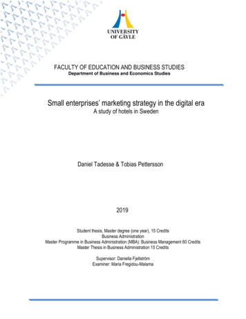
the image containing agent and environment specific information (see Figure 2). This representation allows us to takeadvantage of Convolutional Neural Networks which havebeen shown to work well for image classification tasks [8].The image tensor is of size 4 W H, where W and H arethe height and width of our two dimensional domain andfour is the number of channels in the image. Each channelencodes a different set of information from the global statein its pixel values (shown in Figure 2). The channels can bebroken down in the following way:Improved Agent ironmentobservationFigure 3. Schematic of the multi-agent centralized training process Background Channel: contains information aboutany obstacles in the environment Opponent Channel: contains information about allthe opponentsMulti-Agent Input Ally Channel: contains information about all the allies3x3 conv, 32 Self Channel: contains information about the agentmaking the decision3x3 conv, 32ReLUNote that channels in the image-like representation aresparse. In both the opponent and ally channels, each nonzero pixel value encodes the number of opponents or alliesin that specific position.The second challenge is multi-agent training. When multiple agents are interacting in an environment, their actionsmay directly impact the actions of other agents. To that end,agents must be able to reason about one another in order toact intelligently. In order to incorporate multi-agent training, we train one agent at a time, and keep the policies of allthe other agents fixed during this period. After a set number of iterations the policy learned by the training agent getsdistributed to all the other agents of its type. Specifically, anagent distributes its policy to all of its allies (see Figure 3).This process, allows one set of agents to incrementally improve their policy over time. The learning process itself isnot distributed, since one agent must share its policy withall of its allies. However, the policy execution is distributed,because each agent has their own neural network controller.Each agent must be able to sense the locations of all theother agents, but does not need to explicitly communicatewith the other agents about its intent.The last challenge is dealing with agent ambiguity. Consider a scenario where two ally agents are occupying thesame position in the environment. The image-like state representation for each agent will be identical, so their policieswill be exactly the same. To break this symmetry, we enforce a stochastic policy for our agents. The actions takenby the agent are drawn from a distribution derived by takinga softmax over the Q-values of the neural network. This allows allies to take different actions if they occupy the samestate and break the ambiguity. In previous work, the policy used in evaluation was -greedy [13]. However, a moreBatchNormalization3x3 conv, 32 max pool3x3 conv, 32ReLUBatchNormalization3x3 conv, 32 fc Q-ValuesFigure 5. The multi-agent deep Q-Network (MADQN) architectureprincipled approach would be to use a stochastic policy generated by taking a softmax over the Q-values as proposedhere.3
Background ChannelOpponent ChannelAlly ChannelSelf ChannelFour Channel ImageFigure 2. Four channel image-like representation of the multi-agent state used as input to the deep Q-Network. The background channelencodes the locations of the obstacles in its pixel values, while the ally and opponent channels encode the locations of the allies andopponents. The self channel encodes the location of the agent that is making the decision. Q(a0 )Q(a1 ) Q(a2 )Q-Values ConvolutionFully connectedFigure 4. An example schematic showing the multi-agent image-like state being used as an input to the convolutional neural network.4. Problem Formulation and Network Architecturethe same grid cell as an evader. In this work, we modifythe pursuit-evasion task such that the terminal state of thesystem is reached only when all the evaders are tagged by apursuer. The pursuers receive a large reward in the terminalstate. Thus, in order to reach the high rewarding terminalstate, the pursuers must be able to make decisions in a cooperative manner.To train the neural network controller, the data set containing the image-like state representations was generatedthrough simulation. Specifically, each data sample contained an experience tuple of the form (s, a, r, s0 ), where sis the starting image-like state, a is the action taken, r is thereward received, and s0 is the new state of the system. Aswith other deep reinforcement learning approaches, the experience replay dataset from which the network was trained,was continuously updated during training.The neural network architecture used in this work follows many of the same principles as in previous work [13],with some modifications. Since our state representation isThe primary goal of this work is to evaluate the approachoutlined in the previous section on a simple problem andquantitively identify interesting multi-agent behavior suchas cooperation. To accomplish this, we pick the pursuitevasion problem [3] as our evaluation domain. In pursuitevasion, a set of agents (the pursuers) are attempting tochase another set of agents (the evaders). The agents inthe problem are self-interested (or heterogeneous), i.e. theyhave different objectives. In particular, we focus on computing pursuit policies using the MADRL approach. Specifically, the evaders follow a simple heuristic policy, wherethey move in the direction that takes them furthest from theclosest pursuer. The pursuers are attempting to learn a distributed neural network controller as outlined in the previous section. Since we limit the problem to a discrete statespace, the pursuers receive a reward anytime they occupy4
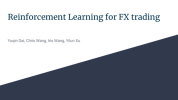
image-like, we can use a convolutional neural network architecture. A schematic of the multi-agent image-like statebeing used as an input to a convolutional neural networkis shown in Figure 4. In the figure, the image-like representation captures all the state information, while the output layer of the network represents the Q-values for all theactions the agent can take from that state. The networkarchitecture used in this work is shown in Figure 5. Thedifferences between this architecture and the architecturesused in previous works is that we adopt the Residual Network [6] architecture or skip connections to improve gradient flow throughout the network, and we use batch normalization. The name of this architecture is multi-agent deepQ-Network or MADQN.bined. We also see that the combined policy can generalizeto scenario where the obstacles are split. While this result ispreliminary, and could be studied with more rigor, it demonstrates that MADQN controllers can generalize well to newenvironments.Next, we evaluated MADQN policies on varying numbers of agents. The results are shown in Figure 8. The figure shows the average reward for a given policy evaluatedon different scenarios. In this evaluation, we consider threetypes policies: N vs N: MADQN policies obtained through trainingon a problem instance with N evaders and N pursuers(e.g. 1 vs 1, 2 vs 2, etc). Heuristic: A heuristic policy in which the pursuermoves towards the evader closest to it.5. ResultsFor the majority of the evaluation, we focused on a10 10 instance of the pursuit-evasion problem with a singlerectangular obstacle in the middle of the environment. Theimage-like states were generated by simulating the motionof the agents, and converting the state into a three dimensional tensor. In this section we provide three experimentalresults that test the capabilities of the MADQN controller.We first demonstrate the ability of the MADQN to generalize to previously unseen environments. Next, we showthat the MADQN can generalize across different numbersof agents. Specifically, we show that MADQN controllersthat have been trained on 2 agent instances can perform wellin 3 agent settings. Lastly, we demonstrate a transfer learning approach for MADQN that speeds up training convergence. During all the evaluations, the initial conditions foreach simulation were set by using rejection sampling. Thestate space was uniformly sampled, and states were rejectedif either agent was inside of an obstacle or if a pursuers wastoo close to an evader (start at least one grid cell away).Figure 6 shows the experimental set-up for MADQNgeneralization over new environments. The figure depictsthe training and evaluation scenarios we used for this experiment. We trained the MADQN on two instances of thepursuit-evasion problem and evaluated on a new instance tosee how well the controller can generalize. Namely, we considered a scenario with a single evader and a single pursuer,on three configurations (Figure 6). The difference betweeneach instance is the obstacle configuration. The MADQNwas trained on the two scenarios shown on the left of Figure 6, and evaluated on the scenario shown on the right ofthe figure. The results are outlined in Table 1. The tableshows evaluation results of both the split policy (policy obtained form training on the two problem instances at once)and the combined policy (policy obtained from training onthe problem instance where the obstacles are combined).We see that the split policy performs just as well as the combined policy on the scenario where the obstacles are com- Value iteration: The optimal policy obtained by solving the multi-agent MDP (tractable only for a scenariowith 1 evader and 1 pursuer)For the N vs N policies, we considered the followingtraining scenarios: 1 vs 1, 2 vs 2 and 3 vs 3. Both the Nvs N and the heuristic policies were evaluated on the following scenarios: 1 vs 1, 2 vs 2, 3 vs 3. We also evaluatedthe value iteration policy on the 1 vs 1 scenario. There arethree main things to take away form the figure. First, all ofthe policies perform near optimally on the 1 vs 1 scenario.Since the value iteration policy servers as an upper boundon performance, we can directly infer that all policies evaluated on the 1 vs 1 scenario have ned-optimal performance.This indicates that the MADQN network can learn near optimal policies for the simple 1 vs 1 scenario. Second, theperformance of the 1 vs 1 and the heuristic policies on the2 vs 2 and the 3 vs 3 scenarios is nearly identical. Sincethe heuristic is just a greedy strategy, this implies that thepolicy learned by the MADQN when trained on the 1 vs 1scenario is similar to the greedy heuristic. This is an important point to consider when evaluating policies that weretrained for more than one agent. In particular, the 1 vs 1policy has no knowledge of cooperation. This can be seenin the evaluation results for the 2 vs 2 and the 3 vs 3 scenarios. Lastly, we compare the performance of the policiestrained on the 2 vs 2 and the 3 vs 3 scenarios against eachother. While the two policies perform best on the scenariosthat they were trained on, both outperform the 1 vs 1 policyon scenario that they were not trained on. For example, the2 vs 2 policy does nearly as well as the 3 vs 3 policy on the 3vs 3 scenario. This implies that the MADQN controllers areable to generalize the notion of cooperation between agentsto different numbers of agents fairly well.In practice training these networks on large problems istime consuming. We explored a transfer learning approachto alleviate some of the computational burden. Figure 85
Table 1. Average rewards per time-step for the pursuit policiesevaluated over 50000 time-steps450Maps0.1640.152Split PolicyCombined .1430.145400350300RewardFlatPolicy Evaluation1 v 1 Policy2 v 2 Policy3 v 3 PolicyHeuristicValue Iteration250200150100No TransferTransfer50000.1550100150Iterations (1000s)200250Figure 8. Evaluation reward for the MADQN during training timefor a 2 vs 2 pursuit-evasion scenario. The green line shows aMADQN initialized with the same weights as a converged 1 vs 1MADQN, while the blue line shows the MADQN initialized withrandom weights.0.100.050.00Transfer Learning Evaluation1v12v2Scenario3v3MADRL, (ii) demonstrated generalization across a varying number of agents using MADRL, and (iii) showed thattransfer learning can be used in multi-agent systems tospeed up convergence.There are a number of potential directions for futurework. While this work considered self-interested agentsimplicitly, their policies were kept stationary. The next stepwould be to train networks that control heterogenous agents.This could be done by having a network for each type ofagent, and alternating training between the networks. Thiswould allow the networks to learn better policies as thebehavior of other types of agents changes in the environment. Another area of future work would involve extendingthis approach to more complicated domains. One potential application is robotic soccer. Specifically, selective coordination approaches have been shown to work well forrobot soccer [11]. Future work will explore if MADRLcan be used to learn policies that perform as well as theselective coordination approaches and if it can outperformthem. Another part of future work is to do a more throughcomparison of the MADRL approach to other multi-agentreinforcement learning techniques such as the minimax Qalgorithm [2]. It may be of value to compare this approachto game theoretic [18] and other reinforcement learning [10]techniques.Figure 7. Average reward per time step for various policies acrossthree different pursuit-evasion scenarios.shows convergence plots for two to MADQNs training onthe 2 vs 2 scenario. The plot shows the average rewardobtained by evaluating each MADQN after a given number of training iterations. The blue curve was generated bytraining a network with random weight initialization (fromscratch). The green curve used the network trained untilconvergence on the 1 vs 1 scenario (transfer network). Thetransfer learning approach of using a network trained on adifferent but related environment allows us to speed up convergence in multi-agent systems. This indicates that we cantrain a single network on a specific problem domain, andif we want to fine tune it for a specific number of agents,we can use transfer learning to quickly improve its performance.6. ConclusionDespite many of the recent advances in optimal control and automated planning, multi-agent systems remainan open research challenge. The difficulties arise from thecurse of dimensionality that makes systems with large numbers of agents intractable. In this work, we demonstratedthat a deep reinforcement learning approach can be usedto solve decision making problems that are intractable forclassical algorithms such as value iteration. The three primary contributions of this work are: (i) demonstrated generalization across environments in multi-agent systems with7. Appendix: Multi-Agent Deep Q-NetworkHyperparametersThe hyperparameters used for training the MADQN canbe found in 2.6
TrainEvaluate Figure 6. Generalization across environments: the multi-agent deep Q-Network was trained on the two pursuit-evasion scenarios on theright, and was evaluated on the scenario on the leftTable 2. Deep Q-Network hyperparametersHyperparameterValueDecriptionMax train iterationsMinimbatch sizeReplay sizeLearning rateUpdate ruleInitial exploration decayTarget network updateAgent network update250000321000000.0001ADAM1.05e-5500050000The maximum number of training samples generatedNumber of training samples per updateSize of the experience replay datasetRate used by the optimizerThe parameter update rule used by the optimizerInitial value in greedy exploration policyRate at which decreasesFrequency of updating the target networkFrequency of updating the networks of other agentsReferences[10] J. Liu, S. Liu, H. Wu, and Y. Zhang. A pursuit-evasionalgorithm based on hierarchical reinforcement learning. InMeasuring Technology and Mechatronics Automation, 2009.ICMTMA’09. International Conference on, volume 2, pages482–486. IEEE, 2009.[11] J. P. Mendoza, J. Biswas, P. Cooksey, R. Wang, S. Klee,D. Zhu, and M. Veloso. Selectively reactive coordinationfor a team of robot soccer champions. In AAAI Conferenceon Artificial Intelligence (AAAI), 2016.[12] V. Mnih, A. P. Badia, M. Mirza, A. Graves, T. P. Lillicrap,T. Harley, D. Silver, and K. Kavukcuoglu. Asynchronousmethods for deep reinforcement learning. arXiv preprintarXiv:1602.01783, 2016.[13] V. Mnih, K. Kavukcuoglu, D. Silver, A. A. Rusu, et al.Human-level control through deep reinforcement learning.Nature, 518(7540):529–533, 02 2015.[14] D. Silver, A. Huang, C. J. Maddison, A. Guez, L. Sifre,G. van den Driessche, J. Schrittwieser, I. Antonoglou,V. Panneershelvam, M. Lanctot, et al. Mastering the gameof go with deep neural networks and tree search. Nature,529(7587):484–489, 2016.[15] A. Tampuu, T. Matiisen, D. Kodelja, I. Kuzovkin, K. Korjus, J. Aru, J. Aru, and R. Vicente. Multiagent cooperationand competition with deep reinforcement learning. CoRR,abs/1511.08779, 2015.[16] J. N. Tsitsiklis and B. Van Roy. An analysis of temporaldifference learning with function approximation. IEEETransactions on Automatic Control, 42(5):674–690, 1997.[17] H. Van Hasselt, A. Guez, and D. Silver. Deep reinforcement learning with double q-learning. arXiv preprintarXiv:1509.06461, 2015.[1] D. S. Bernstein, R. Givan, N. Immerman, and S. Zilberstein.The complexity of decentralized control of Markov decisionprocesses. Mathematics of Operations Research, 27(4):819–840, 2002.[2] L. Busoniu, R. Babuska, and B. De Schutter. A comprehensive survey of multiagent reinforcement learning. Systems,Man, and Cybernetics, Part C: Applications and Reviews,IEEE Transactions on, 38(2):156–172, 2008.[3] T. H. Chung, G. A. Hollinger, and V. Isler. Search andpursuit-evasion in mobile robotics. Autonomous robots,31(4):299–316, 2011.[4] H. Cuayáhuitl, S. Keizer, and O. Lemon. Strategic dialoguemanagement via deep reinforcement learning. arXiv preprintarXiv:1511.08099, 2015.[5] P. J. Gmytrasiewicz and P. Doshi. A framework for sequential planning in multi-agent settings. J. Artif. Intell. Res.(JAIR), 24:49–79, 2005.[6] K. He, X. Zhang, S. Ren, and J. Sun. Deep residual learningfor image recognition. CoRR, abs/1512.03385, 2015.[7] D. Kingma and J. Ba. Adam: A method for stochastic optimization. arXiv preprint arXiv:1412.6980, 2014.[8] A. Krizhevsky, I. Sutskever, and G. E. Hinton. Imagenetclassification with deep convolutional neural networks. InAdvances in Neural Information Processing Systems, page2012, 2012.[9] T. P. Lillicrap, J. J. Hunt, A. Pritzel, N. Heess, T. Erez,Y. Tassa, D. Silver, and D. Wierstra. Continuous control with deep reinforcement learning. arXiv preprintarXiv:1509.02971, 2015.7
[18] R. Vidal, O. Shakernia, H. J. Kim, D. H. Shim, and S. Sastry. Probabilistic pursuit-evasion games: theory, implementation, and experimental evaluation. Robotics and Automation, IEEE Transactions on, 18(5):662–669, 2002.[19] Z. Wang, N. de Freitas, and M. Lanctot. Dueling networkarchitectures for deep reinforcement learning. arXiv preprintarXiv:1511.06581, 2015.8
extending deep reinforcement learning to multi-agent sys-tems. 3.1. Deep Reinforcement Learning In reinforcement learning, an agent interacting with its environment is attempting to learn an optimal control pol-icy. At each time step, the agent observes a state s, chooses an action a, receives a reward r, and transitions to a new state s0. Q .