Transcription
Titlestata.comesize — Effect size based on mean comparisonDescriptionOptionsReferencesQuick startRemarks and examplesAlso seeMenuStored resultsSyntaxMethods and formulasDescriptionesize calculates effect sizes for comparing the difference between the means of a continuousvariable for two groups. In the first form, esize calculates effect sizes for the difference between themean of varname for two groups defined by groupvar. In the second form, esize calculates effectsizes for the difference between varname1 and varname2 , assuming unpaired data.esizei is the immediate form of esize; see [U] 19 Immediate commands. In the first form,esizei calculates the effect size for comparing the difference between the means of two groups. Inthe second form, esizei calculates the effect size for an F test after an ANOVA.Quick startCohen’s d and Hedges’s g comparing the difference in means of v for two independent groups incatvaresize twosample v, by(catvar)As above, but with group data stored in v1 and v2esize unpaired v1 v2As above, but use 90% confidence levelesize unpaired v1 v2, level(90)Cohen’s d and Hedges’s g for means of v for groups in catvar1 calculated over each level ofcatvar2by catvar2: esize twosample v, by(catvar1)MenuesizeStatistics Summaries,tables, and tests Classical tests of hypotheses Effect size based on mean comparisonesizeiStatistics Summaries, tables, and tests Classical tests of hypotheses1 Effect-size calculator
2esize — Effect size based on mean comparisonSyntaxEffect sizes for two independent samples using groups in , by(groupvar) optionsesize twosample varname ifEffect sizes for two independent samples using variables esize unpaired varname1 varname2 ifin , optionsImmediate form of effect sizes for two independent samples esizei # obs1 # mean1 # sd1 # obs2 # mean2 # sd2 , optionsImmediate form of effect sizes for F tests after an ANOVA esizei # df1 # df2 # F , eltapbcorrallunequalwelchlevel(#)report Cohen’s d (1988)report Hedges’s g (1981)report Glass’s (Smith and Glass 1977) using each group’s standard deviationreport the point-biserial correlation coefficient (Pearson 1909)report all estimates of effect sizeuse unequal variancesuse Welch’s (1947) approximationset confidence level; default is level(95)by is allowed with esize, and collect is allowed with esize and esizei; see [U] 11.1.10 Prefix commands.Options Mainby(groupvar) specifies the groupvar that defines the two groups that esize will use to estimate theeffect sizes. Do not confuse the by() option with the by prefix; you can specify both.cohensd specifies that Cohen’s d (1988) be reported.hedgesg specifies that Hedges’s g (1981) be reported.glassdelta specifies that Glass’s (Smith and Glass 1977) be reported.pbcorr specifies that the point-biserial correlation coefficient (Pearson 1909) be reported.all specifies that all estimates of effect size be reported. The default is Cohen’s d and Hedges’s g .unequal specifies that the data not be assumed to have equal variances.welch specifies that the approximate degrees of freedom for the test be obtained from Welch’s formula(1947) rather than from Satterthwaite’s approximation formula (1946), which is the default whenunequal is specified. Specifying welch implies unequal.
esize — Effect size based on mean comparison3level(#) specifies the confidence level, as a percentage, for confidence intervals. The default islevel(95) or as set by set level; see [U] 20.8 Specifying the width of confidence intervals.Remarks and examplesstata.comRemarks are presented under the following headings:IntroductionEstimating effect sizesImmediate formVideo exampleIntroductionWhereas p-values are used to assess the statistical significance of a result, measures of effect sizeare used to assess the practical significance of a result. Effect sizes can be broadly categorized as“measures of group differences” (the d family) and “measures of association” (the r family); seeEllis (2010, table 1.1). The d family includes estimators such as Cohen’s d, Hedges’s g , and Glass’s . The r family includes estimators such as the point-biserial correlation coefficient, η 2 , ε2 , andω 2 (also see estat esize in [R] regress postestimation). For an introduction to the concepts andcalculation of effect sizes, see Kline (2013) and Thompson (2006). For a more detailed discussion, seeKirk (1996), Ellis (2010), Cumming (2012), Grissom and Kim (2012), and Kelley and Preacher (2012).Note that there is much variation in the definitions of measures of effect size (Kline 2013). AsEllis (2010, 27) cautions, “However, beware the inconsistent terminology. What is labeled here as gwas labeled by Hedges and Olkin as d and vice versa. For these authors writing in the early 1980s, gwas the mainstream effect-size index developed by Cohen and refined by Glass (hence g for Glass).However, since then g has become synonymous with Hedges’s equation (not Glass’s) and the reasonit is called Hedges’s g and not Hedges’s h is because it was originally named after Glass—eventhough it was developed by Larry Hedges. Confused?”To avoid confusion, esize and esizei closely follow the notation of Hedges (1981), Smithson (2001), Kline (2013), and Ellis (2010).
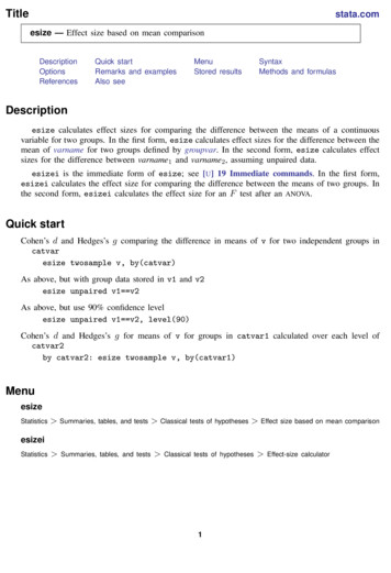
4esize — Effect size based on mean comparisonEstimating effect sizesExample 1: Effect size for two independent samples using by()Suppose we are interested in question 1 from the fictitious depression.dta: “My statisticalsoftware makes me feel sad”. We might have conducted a t test to test the null hypothesis that there isno difference in response by sex. We could then compute various measures of effect size to describethe magnitude of the effect of sex. use ctitious depression inventory data based on the Beck Depression Inventory). esize twosample qu1, by(sex) allEffect size based on mean comparisonObs per group:Female Male Effect 786-.0232208Cohen’sHedges’sGlass’s DeltaGlass’s DeltaPoint-biserial712288[95% conf. s d, Hedges’s g , and both estimates of Glass’s indicate that the score for females is 0.05standard deviations lower than the score for males. The point-biserial correlation coefficient indicatesthat there is a small, negative correlation between the scores for females and males.Technical noteGlass’s has traditionally been estimated for experimental studies using the control group standarddeviation rather than the pooled standard deviation. Kline (2013) notes that the choice of group becomesarbitrary for data arising from observational studies and recommends the reporting of Glass’s usingeach group standard deviation.
esize — Effect size based on mean comparison5Example 2: Effect size for two independent samples by a third variableIf we are interested in the same effect sizes from example 1 stratified by race, we could use theby prefix with the sort option to accomplish this task. by race, sort: esize twosample qu1, by(sex)- race HispanicEffect size based on mean comparisonObs per group:Female Male Effect sizeEstimateCohen’s dHedges’s g-.1042883-.1036899[95% conf. interval]-.463503-.4608434- race BlackEffect size based on mean comparisonObs per group:Female Male Effect sizeEstimateCohen’s dHedges’s g-.1720681-.1717011EstimateCohen’s dHedges’s g.0479511.0478807.2553235.253858425995[95% conf. interval]-.4073814-.4065127- race WhiteEffect size based on mean comparisonObs per group:Female Male Effect size8845.063489.0633536365148[95% conf. interval]-.1430932-.1428831.2389486.2385977
6esize — Effect size based on mean comparisonExample 3: Bootstrap confidence intervals for effect sizesSimulation studies have shown that bootstrap confidence intervals may be preferable to confidenceintervals based on the noncentral t distribution when the variable of interest does not have a normaldistribution (Kelley 2005; Algina, Keselman, and Penfield 2006). Bootstrap confidence intervals canbe easily estimated for effect sizes using the bootstrap prefix. use ctitious depression inventory data based on the Beck Depression Inventory). set seed 12345. bootstrap r(d) r(g), reps(1000) nodots nowarn: esize twosample qu1, by(sex)Bootstrap resultsNumber of obs 1,000Replications 1,000Command: esize twosample qu1, by(sex)bs 1: r(d)bs 2: r(g)bs 1bs 2ObservedcoefficientBootstrapstd. ormal-based[95% conf. interval]P z e 4: Effect sizes for two independent samples using variablesSometimes, the data of interest are stored in two separate variables. We can calculate effect sizesfor the two groups by using the unpaired version of esize. use https://www.stata-press.com/data/r17/fuel. esize unpaired mpg1 mpg2Effect size based on mean comparisonNumber of obs Effect sizeEstimateCohen’s dHedges’s g-.5829654-.562824324[95% conf. interval]-1.394934-1.34674.2416105.2332631
esize — Effect size based on mean comparison7Immediate formExample 5: Immediate form for effect sizes for two meansOften we do not have access to raw data, but we are given summary statistics in a report ormanuscript. To calculate the effect sizes from summary statistics, we can use the immediate commandesizei. For example, Kline (2013) in table 4.2 shows summary statistics for a hypothetical samplewhere mean1 13, sd1 2.74, mean2 11, and sd2 2.24; there are 30 people in each group.We can estimate the effect sizes from these summary data using esizei:. esizei 30 13 2.74 30 11 2.24Effect size based on mean comparisonObs per group:Group 1 Group 2 3030Effect sizeEstimate[95% conf. interval]Cohen’s dHedges’s xample 6: Immediate form for effect sizes for F tests after an ANOVAesizei can also be used to compute η 2 , ε2 , and ω 2 for F tests after an ANOVA. The followingexample from Smithson (2001, 623) illustrates the use of esizei for dfnum 4, dfden 50, andF 4.2317:. esizei 4 50 4.2317, level(90)Effect sizes for linear modelsEffect sizeEstimate[90% conf. 529151.1931483.1903049.0521585Video exampleTour of effect sizes.3603621
8esize — Effect size based on mean comparisonStored resultsesize and esizei for comparing two means store the following in r():Scalarsr(d)r(lb d)r(ub d)r(g)r(lb g)r(ub g)r(delta1)r(lb delta1)r(ub delta1)r(delta2)r(lb delta2)r(ub delta2)r(r pb)r(lb r pb)r(ub r pb)r(N 1)r(N 2)r(df t)r(level)Cohen’s dlower confidence bound for Cohen’s dupper confidence bound for Cohen’s dHedges’s glower confidence bound for Hedges’s gupper confidence bound for Hedges’s gGlass’s for group 1lower confidence bound for Glass’s for group 1upper confidence bound for Glass’s for group 1Glass’s for group 2lower confidence bound for Glass’s for group 2upper confidence bound for Glass’s for group 2point-biserial correlation coefficientlower confidence bound for the point-biserial correlation coefficientupper confidence bound for the point-biserial correlation coefficientsample size n1sample size n2degrees of freedomconfidence levelesizei for F tests after ANOVA stores the following in r():Scalarsr(eta2)r(lb eta2)r(ub eta2)r(epsilon2)r(omega2)r(level)η2lower confidence bound for η 2upper confidence bound for η 2ε2ω2confidence levelMethods and formulasFor the d family, the effect-size parameter of interest is the scaled difference between the meansgiven by(µ1 µ2 )δ σOne of the most popular estimators of effect size is Cohen’s d, given byCohen’s d wheress (x1 x2 )s (n1 1)s21 (n2 1)s22n1 n2 2
esize — Effect size based on mean comparison9Hedges (1981) showed that Cohen’s d is biased and proposed the unbiased estimatorHedges’s g Cohen’s d c(m)where m n1 n2 2 and Γ m2 pc(m) mm 12Γ2Glass (Smith and Glass 1977) proposed an estimator for δ in the context of designed experiments,Glass’s (xtreated xcontrol )scontrolwhere scontrol is the standard deviation for the control group.As noted above, esize and esizei report two estimates of Glass’s : one using the standarddeviation for group 1 and the other using the standard deviation for group 2:Glass’s 1 (x1 x2 )s1Glass’s 2 (x1 x2 )s2andFor the r family, the effect-size parameter of interest is the ratio of the variance attributable to aneffect and the total variance:σ2η 2 effect2σtotalA popular estimator of η when there are two groups is the point-biserial correlation coefficient,rPB t2t dfwhere t is the t statistic for the difference between the means of the two groups, and df is thecorresponding degrees of freedom. Satterthwaite’s or Welch’s adjustment (see [R] ttest for details) tothe degrees of freedom can be used to calculate rPB by specifying the unequal or welch option,respectively.When more than two means are being compared, as in the case of an ANOVA with p groups,a popular estimator of effect size is the correlation ratio denoted η 2 (Fisher 1925; Kerlinger andLee 2000). η 2 can be computed directly as the ratio of the SSeffect and the SStotal or as a functionof the F statistic with numerator degrees of freedom equal to dfnum and denominator degrees offreedom equal to dfden .Fηb2 F dfden /dfnumLike its equivalent estimator R2 , η 2 has an upward bias. Less biased estimators of effect size areε and ω 2 (Grissom and Kim 2012).2εb2 F 1dfnum ηb2 (1 ηb2 )F dfden /dfnumdfden
10esize — Effect size based on mean comparisonωb2 F 1F (dfden 1)/dfnumTo calculate ηb2 , εb2 , and ωb 2 directly after anova or regress, see estat esize in [R] regresspostestimation.Cohen’s d, Hedges’s g , and Glass’s have been shown to have a noncentral t distribution(Hedges 1981) with noncentrality parameter equal torλ δn1 n2n1 n2Confidence intervals are calculated by finding the noncentrality parameters λlower and λupper thatcorrespond toαPr(df, δ, λlower ) 1 2andPr(df, δ, λupper ) α2using the function npnt(df ,t,p). The noncentrality parameters are then transformed back to theeffect-size scale:rn1 n2δlower λlowern1 n2andrδupper λuppern1 n2n1 n2(see Venables [1975]; Steiger and Fouladi [1997]; Cumming and Finch [2001]; Smithson [2001]).Confidence intervals for the point-biserial correlation coefficient are calculated similarly andtransformed back to the effect-size scale asλlowerrlower p 2λlower dfandλupperrupper qλ2upper dfFollowing Smithson’s (2001) notation, the F statistic is written asFdfnum ,dfden f 2 (dfnum /dfden )This equation has a noncentral F distribution with noncentrality parameter:λ f 2 (dfnum dfden 1)where f 2 η 2 /(1 η 2 ).
esize — Effect size based on mean comparison11Confidence intervals for ηb2 are calculated by finding the noncentrality parameters λlower andλupper for a noncentral F distribution that correspond toPr(dfnum , dfden , F, λlower ) 1 α2andα2using the function npnF(df1 ,df2 ,f ,p). The noncentrality parameters are transformed back to theηb2 scale asλlower2ηblower λlower dfnum dfden 1Pr(dfnum , dfden , F, λupper ) and2ηbupper λupperλupper dfnum dfden 1While confidence intervals for εb2 can be constructed using the same transformation that links it withηb2 , there are several arguments for not using them in practice. See Smithson (2003, 54) for furtherdetails. Fred Nichols Kerlinger (1910–1991) was born in New York City. He studied music at NewYork University and graduated magna cum laude with a degree in education and philosophy.After graduation, he joined the U.S. Army and served as a counterintelligence officer in Japanin 1946. Kerlinger earned an MA and a PhD in educational psychology from the University ofMichigan and held faculty appointments at several universities, including New York University.He was president of the American Educational Research Association and is best known forhis popular and influential book Foundations of Behavioral Research (1964), which introducedFisher’s (1925) η 2 statistic to behavioral researchers. William Lee Hays (1926–1995) was born in Clarksville, Texas. He studied mathematics andpsychology at Paris Junior College in Paris, Texas, and at East Texas State College. He earned BSand MS degrees from North Texas State University. Upon completion of his PhD in psychologyat the University of Michigan, he joined the faculty, where he eventually became associate vicepresident for academic affairs. In 1977, Hays accepted an appointment as vice president foracademic affairs at the University of Texas at Austin, where he remained until his death in 1995.Hays is best known for his book Statistics for Psychologists (1963), which introduced the ω 2statistic (and is actually denoted here by ε2 ). ReferencesAlgina, J., H. J. Keselman, and R. D. Penfield. 2006. Confidence interval coverage for Cohen’s effect size statistic.Educational and Psychological Measurement 66: 945–960. https://doi.org/10.1177/0013164406288161.Baldwin, S. 2019. Psychological Statistics and Psychometrics Using Stata. College Station, TX: Stata Press.Cohen, J. 1988. Statistical Power Analysis for the Behavioral Sciences. 2nd ed. Hillsdale, NJ: Erlbaum.Cumming, G. 2012. Understanding the New Statistics: Effect Sizes, Confidence Intervals, and Meta-Analysis. NewYork: Routledge.Cumming, G., and S. Finch. 2001. A primer on the understanding, use, and calculation of confidence intervalsthat are based on central and noncentral distributions. Educational and Psychological Measurement 61: .
12esize — Effect size based on mean comparisonEllis, P. D. 2010. The Essential Guide to Effect Sizes: Statistical Power, Meta-Analysis, and the Interpretation ofResearch Results. Cambridge: Cambridge University Press.Fisher, R. A. 1925. Statistical Methods for Research Workers. Edinburgh: Oliver & Boyd.Grissom, R. J., and J. J. Kim. 2012. Effect Sizes for Research: Univariate and Multivariate Applications. 2nd ed.New York: Routledge.Hays, W. L. 1963. Statistics for Psychologists. New York: Holt, Rinehart & Winston.Hedges, L. V. 1981. Distribution theory for Glass’s estimator of effect size and related estimators. Journal of EducationalStatistics 6: 107–128. https://doi.org/10.2307/1164588.Huber, C. 2013. Measures of effect size in Stata 13. The Stata Blog: Not Elsewhere es-of-effect-size-in-stata-13/.Kelley, K. 2005. The effects of nonnormal distributions on confidence intervals around the standardized meandifference: Bootstrap and parametric confidence intervals. Educational and Psychological Measurement 65: lley, K., and K. J. Preacher. 2012. On effect size. Psychological Methods 17: er, F. N. 1964. Foundations of Behavioral Research. New York: Holt, Rinehart & Winston.Kerlinger, F. N., and H. B. Lee. 2000. Foundations of Behavioral Research. 4th ed. Belmont, CA: Wadsworth.Kirk, R. E. 1996. Practical significance: A concept whose time has come. Educational and Psychological Measurement56: 746–759. https://doi.org/10.1177/0013164496056005002.Kline, R. B. 2013. Beyond Significance Testing: Statistics Reform in the Behavioral Sciences. 2nd ed. Washington,DC: American Psychological Association.Miller, D. J., J. T. Nguyen, and M. Bottai. 2020. emagnification: A tool for estimating effect-size magnification andperforming design calculations in epidemiological studies. Stata Journal 20: 548–564.Pearson, K. 1909. On a new method of determining correlation between a measured character A, and a character B,of which only the percentage of cases wherein B exceeds (or falls short of) a given intensity is recorded for eachgrade of A. Biometrika 7: 96–105. http://doi.org/10.2307/2345365.Satterthwaite, F. E. 1946. An approximate distribution of estimates of variance components. Biometrics Bulletin 2:110–114. https://doi.org/10.2307/3002019.Shaw, B. P. 2022. Effect sizes for contrasts of estimated marginal effects. Stata Journal 22: 134–157.Smith, M. L., and G. V. Glass. 1977. Meta-analysis of psychotherapy outcome studies. American Psychologist 32:752–760. , M. 2001. Correct confidence intervals for various regression effect sizes and parameters: The importanceof noncentral distributions in computing intervals. Educational and Psychological Measurement 61: 2. 2003. Confidence Intervals. Thousand Oaks, CA: SAGE.Steiger, J. H., and R. T. Fouladi. 1997. Noncentrality interval estimation and the evaluation of statistical models. InWhat If There Were No Significance Tests?, ed. L. L. Harlow, S. A. Mulaik, and J. H. Steiger, 221–257. Mahwah,NJ: Erlbaum.Thompson, B. 2006. Foundations of Behavioral Statistics: An Insight-Based Approach. New York: Guilford Press.Venables, W. 1975. Calculation of confidence intervals for noncentrality parameters. Journal of the Royal StatisticalSociety, Series B 37: 406–412. .Welch, B. L. 1947. The generalization of ‘student’s’ problem when several different population variances are involved.Biometrika 34: 28–35. https://doi.org/10.2307/2332510.
esize — Effect size based on mean comparisonAlso see[R] bitest — Binomial probability test[R] ci — Confidence intervals for means, proportions, and variances[R] mean — Estimate means[R] oneway — One-way analysis of variance[R] prtest — Tests of proportions[R] sdtest — Variance-comparison tests[R] ttest — t tests (mean-comparison tests)13
Point-biserial r -.0232208 -.0849629 .0387995 Cohen's d, Hedges's g, and both estimates of Glass's indicate that the score for females is 0.05 standard deviations lower than the score for males. The point-biserial correlation coefficient indicates that there is a small, negative correlation between the scores for females and males.