Transcription
BIOSTATS 640 – Spring 20186. Survival AnalysisStata Illustration6. Introduction to Survival AnalysisIllustration – Stata version 15April 20181. Illustration: DPCA Study of Primary Biliary Cirrhosis 22. Prepare Data for Survival Analysis . .33. Model Free Approaches . a. Descriptives .b. Kaplan-Meier Curve Estimation . .c. Kaplan-Meier Curve Plot . .d. Log Rank Test for Equality of Survival Distributions . . .446784. Cox PH Model Regression . .a. Fit Cox PH Model .b. Multivariable Model Development .c. Side-by-side Comparison of Models .9912125. Regression Diagnostics for Cox PH Model . .a. Test of Proportional Hazards . . .b. Graphical Assessment of Proportional Hazards .c. Test of Overall Goodness-of-Fit . .14141416 .Stata\00. Stata Handouts 2017-18\Stata for Survival Analysis.docxPage 1 of 16
BIOSTATS 640 – Spring 20186. Survival AnalysisStata Illustration1. IllustrationDPCA Study of Primary Biliary CirrhosisPreliminary – Download the stata data set pbc.dta.(a) Direct entry from the internet using the command useuse ta”, clear(b) Download from course website to desk top followed by FILE OPENThe dataset pbc.dta can be found in two /webpages/survival.htmDPCA Study of Primary Biliary Cirrhosissource:Dickson ER, Grambsch PM and Fleming TR (1989) Prognosis in primary biliary-cirrhosis - model for decision making. Hepatology, 10, 1-7.Introduction.Bile is a fluid produced in your liver which functions in the digestion of food and, in aids in ridding your body ofworn-out red blood cells, cholesterol and toxins. The disease primary biliary cirrhosis is an autoimmune disease inwhich the body turns against its own cells, in this case bile ducts. As the bile ducts are increasingly damaged, harmfulsubstances can accumulate. This can lead to irreversible scarring of liver tissue (this is cirrhosis). Among otherthings, the sufferer can experience abdominal pain, internal bleeding and, ultimately, liver failure. Primary biliarycirrhosis is also a risk factor for liver cancer.This illustration utilizes data from a randomized controlled trial of D-penicillamine (DPCA) for the treatment ofprimary biliary cirrhosis. A total of n 312 consenting subjects were enrolled and randomized to either activetreatment or placebo-control (presumably this group received standard care). Time zero is date of diagnosis andinitiation of treatment. Study participants were followed to event of end-stage liver disease or censoring. Thus, theseare an example of “right” censored data. Over the approximate 10 years of follow-up, 125 events of death (40%) wereobserved.The goal of these analyses was to assess the benefit of randomization to DPCA on survival, overall and afteradjustment for selected, important, covariates.Data Dictionary/Coding Manual.This illustration utilizes the following variables in sContinuous (range: 0.11 – 12.47)1 dead0 censored1 DPCA 0 Control1 lowest, 2, 3, 4 highestContinuous, mg/dl .Stata\00. Stata Handouts 2017-18\Stata for Survival Analysis.docxLabelTime to death (in years)Event/censoring indicatorTreatment/randomizationSeverity of liver damage at dxSerum bilirubinPage 2 of 16
BIOSTATS 640 – Spring 20186. Survival AnalysisStata Illustration2. Prepare Data for Survival Analysis. use "/Users/cbigelow/Desktop/pbc.dta"(PBC Natural Hx Data). * Check data set (variables of interest only). codebook years status rx histol bilirubin, compactVariableObs UniqueMeanMinMax ---------years3123015.49312 .1122519 12.47365 Time to Death (in Years)status3122.40064101 Alive/Deadrx3122 .493589701 treatmenthistol3124 3.03205114 Histologic stage of diseasebilirubin 312853.25609.328 Serum Bilirubin in ----------.* ---- Declare Data to be Survival Data ------** Time to event: years* Censoring: status (1 dead, 0 censored)* Command is stset TIMETOEVENT, failure(CENSORVARIABLE). stset years, failure(status)failure event:obs. time interval:exit on or before:status ! 0 & status .(0, ----------------------------------------312 total observations0 -------------------------------------312 observations remaining, representing125 failures in single-record/single-failure data1713.854 total analysis time at risk and under observationat risk from t 0earliest observed entry t 0last observed exit t 12.47365. * Describe survival data using command stsum. stsumfailure d:analysis time t:statusyears incidenceno. of ------ Survival time ----- time at riskratesubjects25%50%75%--------- ------------------total 1713.853528.07293513124.071184 9.295004.Interpretation: The 25th and 50th percentiles of survival are shown. The 25th percentile is 4.07 years and says that 25% of participants have survival times less than4.07 years. The missing value for the 75th percentile is the result of the high prevalence of censoring in this cohort. .Stata\00. Stata Handouts 2017-18\Stata for Survival Analysis.docxPage 3 of 16
BIOSTATS 640 – Spring 20186. Survival AnalysisStata Illustration3. Model Free Approachesa. Descriptives. * Continuous variables. sort rx. tabstat years bilirubin, by(rx) statistics(n mean sd min q max) columns(statistics) format(%8.2f)longstubrxvariable Nmeansdminp25p50p75max--------------------- -----------------------------Placeboyears 158.005.523.000.113.375.197.2412.47bilirubin ------ -----------------------------DPCAyears 154.005.473.160.143.154.967.5912.38bilirubin ------ -----------------------------Totalyears 312.005.493.080.113.265.047.4012.47bilirubin -------------------------------------. * Discrete variables. fre rx histol statusrx -- --------------------- Freq.PercentValidCum.------------------ -------------------------------------------Valid0 Placebo 15850.6450.6450.641 DPCA 15449.3649.36100.00Total ---------------------------histol -- Histologic stage of --------------- Freq.PercentValidCum.-------------- -------------------------------------------Valid1 165.135.135.132 6721.4721.4726.603 12038.4638.4665.064 10934.9434.94100.00Total -----------------------status -- ----------------------- Freq.PercentValidCum.------------------- -------------------------------------------Valid0 Censored 18759.9459.9459.941 Dead 12540.0640.06100.00Total ----------------------------- .Stata\00. Stata Handouts 2017-18\Stata for Survival Analysis.docxPage 4 of 16
BIOSTATS 640 – Spring 20186. Survival AnalysisStata Illustration. tab2 rx status, row column- tabulation of rx by status ------------------- Key ------------------- frequency row percentage column percentage ------------------- Alive/Deadtreatment CensoredDead Total----------- ---------------------- ---------Placebo 9365 158 58.8641.14 100.00 49.7352.00 50.64----------- ---------------------- ---------DPCA 9460 154 61.0438.96 100.00 50.2748.00 49.36----------- ---------------------- ---------Total 187125 312 59.9440.06 100.00 100.00100.00 100.00Interpretation:Among n 158 randomized to PLACEBO, there were 65 deaths (41%)Among n 154 randomized to active treatment DPCA, there were 60 deaths (40%) .Stata\00. Stata Handouts 2017-18\Stata for Survival Analysis.docxPage 5 of 16
BIOSTATS 640 – Spring 20186. Survival AnalysisStata Illustrationb. Kaplan-Meier Curve EstimationNote – must have previously issued command stset to declare data as survival data see again, page 3). * Single Group Kaplan-Meier Curve Estimation. * Command is sts list. sts listfailure d:analysis time t:statusyearsKaplan- Meier ionError[95% Conf. 20.00640.96620.9952---rows omitted -----. * Two Group Kaplan-Meier Curve Estimation. * Command is sts list, by(GROUPVAR)Note:. sort rx. sts list, by(rx)failure d: statusanalysis time t: yearsMust have sorted by GROUPVAR firstKaplan- Meier ionError[95% Conf. 100.97470.01250.93400.9904---- rows omitted 70.9937---- rows omitted ------------------------------ .Stata\00. Stata Handouts 2017-18\Stata for Survival Analysis.docxPage 6 of 16
BIOSTATS 640 – Spring 20186. Survival AnalysisStata Illustrationc. Kaplan-Meier Curve Plot. * ---- Single Group:Kaplan Meier Curve---*. * --- no frills plot --*. sts graph. * with frills --*. sts graph, xlabel(0(1)13) ylabel(0(.20)1) xtitle("Years Since Diagnosis") ytitle("KM Estimated PercentAlive") title("DPCA Study of Primary Biliary Cirrhosis") subtitle("n 312, # events 125")caption("graph02.png", size(vsmall)). * With Greenwood CI limits. sts graph, gwood legend(off) xlabel(0(1)13) ylabel(0(.20)1) xtitle("Years Since Diagnosis") ytitle("KMEstimated Percent Alive (95%CI)") title("DPCA Study of Primary Biliary Cirrhosis") subtitle("n 312, #events 125") caption("graph03.png", size(vsmall))No Frills .Stata\00. Stata Handouts 2017-18\Stata for Survival Analysis.docxWith FrillsWith Greenwood CI LimitsPage 7 of 16
BIOSTATS 640 – Spring 20186. Survival Analysis. * Two Group Kaplan-Meier Curve Estimation. * Command is sts graph, by(GROUPVAR) OPTION OPTION OPTION. sort rx. sts list, by(rx)Stata IllustrationNote:Must have sorted by GROUPVAR first. * with frills ---*. sts graph, by(rx) xlabel(0(1)13) ylabel(0(.20)1) xtitle("Years Since Diagnosis") ytitle("KM EstimatedPercent Alive") title("DPCA Study of Primary Biliary Cirrhosis") subtitle("n 312, # events 125")caption("graph04.png", size(vsmall))d. Log Rank Test of Equality of Survival Distributions. * ---- Log Rank Test (NULL: equality of survival distributions among rx groups). * Command is sts test GROUPVAR. sts test rxfailure d:analysis time t:statusyearsLog-rank test for equality of survivor functions EventsEventsrx observedexpected-------- ------------------------Placebo 6563.22DPCA 6061.78-------- ------------------------Total 125125.00chi2(1) Pr chi2 0.100.7498Interpretation: Do NOT reject. Assumption of the null hypothesis has NOT led to an unlikely result (p-value .75). We have no statistically significant evidence thatthe survival distributions are not the same. .Stata\00. Stata Handouts 2017-18\Stata for Survival Analysis.docxPage 8 of 16
BIOSTATS 640 – Spring 20186. Survival AnalysisStata Illustration4. Cox PH Model RegressionRecall. The Cox PH model models the hazard of event (in this case death) at time “t” as the product of a baselinehazard times exp(linear model in the predictors X1, X2, . Xp). Here, p 3 because we have 3 predictors ofinterest:h(t; X1 ,.X p ) h 0 (t) exp[ β1X1 . β p X p ]X1 rx , 0/1 indicator of randomizationX2 histol, ordinal measure of degree of tissue damage at diagnosisX3 bilirubin, continuous (mg/dl)Note. The predictor histol is an ordinal predictor. So we will need to replace it with appropriately defineddesign variables prior to modeling.a. Fit Cox PH Model. * Single Predictor Model:. stcox rxrx (User coded as 0/1 already)Cox regression -- Breslow method for tiesNo. of subjects No. of failures Time at risk Log likelihood 3121251713.853528-639.92903Number of obs 312LR chi2(1)Prob chi2 ------------------------------------- t Haz. RatioStd. Err.zP z [95% Conf. Interval]------------- -------------rx -------------------Interpretation: Relative to control patients, patients treated with DPCA have lower hazard of death (HR .94) at all times of follow-up. This very small benefit is notstatistically significant (p-value .75). Notice that the 95% CI for the HR includes the null value of 1. * Single Predictor Model:. stcox i.rxrx (Stata defined design variable)Cox regression -- Breslow method for tiesNo. of subjects No. of failures Time at risk Log likelihood 3121251713.853528-639.92903Number of obs 312LR chi2(1)Prob chi2 ------------------------------------- t Haz. RatioStd. Err.zP z [95% Conf. Interval]------------- -------------rx DPCA -------------------Interpretation: SAME. Relative to control patients, patients treated with DPCA have lower hazard of death (HR .94) at all times of follow-up. This very smallbenefit is not statistically significant (p-value .75). Notice that the 95% CI for the HR includes the null value of 1. .Stata\00. Stata Handouts 2017-18\Stata for Survival Analysis.docxPage 9 of 16
BIOSTATS 640 – Spring 2018. * Single Predictor Model:6. Survival AnalysisStata Illustrationhistol (user created design variables). generate histol2 0. replace histol2 1 if histol 2(67 real changes made). generate histol3 0. replace histol3 1 if histol 3(120 real changes made). generate histol4 0. replace histol4 1 if histol 4(109 real changes made). stcox histol2 histol3 histol4failure d:analysis time t:statusyearsCox regression -- Breslow method for tiesNo. of subjects No. of failures Time at risk Log likelihood3121251713.853528 -613.62114Number of obs 312LR chi2(3)Prob chi2 -------------------------------------- t Haz. RatioStd. Err.zP z [95% Conf. Interval]------------- -------------histol2 4.9879765.1431531.560.119.661061137.63631histol3 8.5803218.6853712.120.0341.17999662.39165histol4 ------------------Interpretation: Recall. Higher score on histol (valid scores 1, 2, 3, 4) represent greater level of liver tissue damage present at diagnosis. This model shows thathigher (“worse”) values of histol at diagnosis are associated with poorer prognosis (Hazard ratio estimates increase from 1 to 4.98 to 8.58 to 21.4, relative to the referentgroup histol 1). This is highly statistically significant. Caveat: Note that the confidence intervals are wide. * Single Predictor Model:. stcox i.histolfailure d:analysis time t:histol (Stata generated design variables)statusyearsCox regression -- Breslow method for tiesNo. of subjects No. of failures Time at risk Log likelihood 3121251713.853528-613.62114Number of obs 312LR chi2(3)Prob chi2 -------------------------------------- t Haz. RatioStd. Err.zP z [95% Conf. Interval]------------- -------------histol 2 4.9879765.1431531.560.119.661061137.636313 8.5803218.6853712.120.0341.17999662.391654 ------------------Interpretation: SAME. Higher (“worse”) values of histol at diagnosis are associated with poorer prognosis (Hazard ratio estimates increase from 1 to 4.98 to 8.58 to21.4, relative to the referent group histol 1). This is highly statistically significant. Caveat: Note that the confidence intervals are wide. .Stata\00. Stata Handouts 2017-18\Stata for Survival Analysis.docxPage 10 of 16
BIOSTATS 640 – Spring 2018. * Single Predictor Model:. stcox bilirubinfailure d:analysis time t:6. Survival AnalysisStata IllustrationbilirubinstatusyearsIteration 0:log likelihoodIteration 1:log likelihoodIteration 2:log likelihoodIteration 3:log likelihoodRefining estimates:Iteration 0:log likelihood -639.97989 -611.85115 -597.6878 -597.6845 -597.6845Cox regression -- Breslow method for tiesNo. of subjects No. of failures Time at risk Log likelihood3121251713.853528 -597.6845Number of obs 312LR chi2(1)Prob chi2 -------------------------------------- t Haz. RatioStd. Err.zP z [95% Conf. Interval]------------- -------------bilirubin -------------------Interpretation: Associated with each 1 unit (1 mg/dl) increase in bilirubin is an increased risk of death at all times of follow-up (HR 1.16, 95% CI 1.13 – 1.19). Thisis highly statistically significant (p-value .0001). * Use option nohr to obtain betas instead of hazard ratios. stcox bilirubin, nohrfailure d:analysis time t:statusyearsCox regression -- Breslow method for tiesNo. of subjects No. of failures Time at risk Log likelihood 3121251713.853528-597.6845Number of obs 312LR chi2(1)Prob chi2 -------------------------------------- t Coef.Std. Err.zP z [95% Conf. Interval]------------- -------------bilirubin -------------------- .Stata\00. Stata Handouts 2017-18\Stata for Survival Analysis.docxPage 11 of 16
BIOSTATS 640 – Spring 20186. Survival AnalysisStata Illustrationb. Multivariable Model Development. *------------LR Tests---------*. * --- rx controlling for histol ------*. quietly: stcox i.histol. eststo model histol. quietly: stcox i.histol i.rx. eststo model histolrx. lrtest model histol model histolrxLikelihood-ratio test(Assumption: model histol nested in model histolrx)LR chi2(1) Prob chi2 0.670.4138Interpretation: Do not reject. After adjustment for histol, randomization to DPCA is NOT associated with survival (LR Test p-value .41). * --- rx controlling for bilirubin ------*. quietly: stcox bilirubin. eststo model bili. quietly: stcox bilirubin i.rx. eststo model bilirx. lrtest model bili model bilirxLikelihood-ratio test(Assumption: model bili nested in model bilirx)LR chi2(1) Prob chi2 1.200.2732Interpretation: Do not reject. After adjustment for bilirubin, randomization to DPCA is NOT associated with survival (LR Test p-value .27). * --- rx controlling for both histol and bilirubin. quietly: stcox i.histol bilirubin. eststo model both. quietly: stcox i.histol bilirubin i.rx. eststo model bothrx. lrtest model both model bothrxLikelihood-ratio test(Assumption: model both nested in model bothrx)LR chi2(1) Prob chi2 0.760.3837Interpretation: Do not reject. After adjustment for both histol and bilirubin, randomization to DPCA is NOT associated with survival (LR Test p-value .38)c. Side-by-side Comparison of Models. quietly: stcox i.rx. eststo model1. quietly: stcox bilirubin i.rx. eststo model2. quietly: stcox i.histol i.rx. eststo model3. quietly: stcox bilirubin i.histol i.rx. eststo model4 .Stata\00. Stata Handouts 2017-18\Stata for Survival Analysis.docxPage 12 of 16
BIOSTATS 640 – Spring 20186. Survival AnalysisStata Illustration. * Display Betas and Summary Statistics. estout model1 model2 model3 model4, stats(n chi2 bic, star(chi2)) ---------------------------------KEY:Chi2 Value of LR test comparing the model fit (“full”) to intercept only (“reduced”)bic Schwarz’ Bayesian Information Criterion It is a function of the log-likelihood. Smaller values indicate a better fit. * Display Hazard Ratios and Model Fit Statistics. Option eform produces hazard ratios *. estout model1 model2 model3 model4, eform stats(n chi2 bic, star(chi2)) prehead("Hazard Ratios")Hazard ------------------ .Stata\00. Stata Handouts 2017-18\Stata for Survival Analysis.docxPage 13 of 16
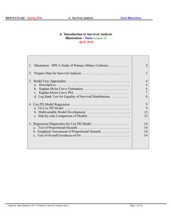
BIOSTATS 640 – Spring 20186. Survival AnalysisStata Illustration5. Regression Diagnostics for Cox PH Modela. Test of Proportional Hazards. * Test of proportional hazards. quietly: stcox bilirubin i.histol i.rx. estat phtest, detailTest of proportional-hazards assumptionTime: ----------------- rhochi2dfProb chi2------------ bilirubin 0.096860.8810.34851b.histol .1.2.histol 0.017750.0410.84243.histol 0.001870.0010.98344.histol -0.048110.2910.59140b.rx .1.1.rx -0.090260.9910.3204------------ global test -------------------------Interpretation: The global test is significant (p-value - .02) but .For each predictor, do not reject the assumption of proportional hazardsb. Graphical Assessment of Proportional Hazards. * Assessment of PH Assumption: Randomization/Treatment. stphplot, by(rx) adjust(bilirubin histol) nolntime plot1opts(symbol(none) color(red) lpattern(dash))plot2opts(symbol(none) color(navy)) title("Assessment of PH Assumption") subtitle(" Predictor is rx") xtitle("Years")Interpretation: Looks reasonable.Note: adjust(bilirubin histol) tells Stata to set these variables to their mean valuesThe option nolntime tells Stata to plot time on the horizontal, not the logarithm of time. .Stata\00. Stata Handouts 2017-18\Stata for Survival Analysis.docxPage 14 of 16
BIOSTATS 640 – Spring 20186. Survival AnalysisStata Illustration. * Assessment of PH Assumption: Histol. stphplot, by(histol) adjust(bilirubin rx) nolntime plot1opts(symbol(none) color(black) lpattern(dash)) plot2opts(symbol(none) color(navy)) plot3opts(symbol(none) color(green)) plot4opts(symbol(none) color(red)) title("Assessment ofPH Assumption") subtitle(" Predictor is histol") xtitle("Years")Interpretation: Looks reasonable, except for the group, histol 1. I checked on this (not shown); there was just 1 death in this group. * Assessment of PH Assumption:Bilirubin, using Quartile Groupings. centile bilirubin, c(25,50,75)-- Binom. Interp. -Variable Obs PercentileCentile[95% Conf. Interval]------------- ----------bilirubin 31225.8.7.9 501.351.21.8 753.4753.126354.5. generate bilicat bilirubin. recode bilicat (min/0.8 1) (0.81/1.35 2) (1.351/3.475 3) (3.4751/max 4) if bilirubin ! .(bilicat: 307 changes made). stphplot, by(bilicat) adjust(rx) nolntime plot1opts(symbol(none) color(black) lpattern(dash)) plot2opts(symbol(none)color(navy)) plot3opts(symbol(none) color(green)) plot4opts(symbol(none) color(red)) title("Assessment of PHAssumption") subtitle(" Predictor is Quartile of Bilirubin") xtitle("Years")Interpretation: Looks reasonable. .Stata\00. Stata Handouts 2017-18\Stata for Survival Analysis.docxPage 15 of 16
BIOSTATS 640 – Spring 20186. Survival AnalysisStata Illustrationc. Test of Overall Goodness of FitNote #1. This test utilizes a command stcoxgof that must be downloaded from the internetNote #2. The command stcoxgof will not work with factor variables. Therefore, in fitting my model, I replacedhistol with the 0/1 indicators of levels 2, 3, and 4. See again page 10.Note #3. The command stcoxgof also requires that you have saved thie martingale residuals. This isaccomplished with the option mgale(NAMEYOUPROVIDE). findit stcoxgof----- not shown:Downloading of stcoxgof---. stcox bilirubin histol2 histol3 histol4 rx, mgale(mgale). stcoxgofGoodness-of-fit test for the inclusion of design variables based on 3 quantiles of risk(Added variables version of the Groennesby and Borgan test)Score testchi2(2) Prob chi2 2.3180.3137Likelihood-ratio testLR chi2(2) Prob chi2 2.3560.3079(Tablecollapsed on quantiles of linear ---------------------------------------Quantile of Risk ObservedExpectedzp-NormObservations---------- ------------------1 1922.87-.809.4181082 3634.409.271.7861023 7067.721.277.782102 Total on: Good. Do not reject. We do not have statistically significant evidence of a poor fit (p-value .31).Caveat: It is quite possible that that additional regression diagnostics will reveal issues! .Stata\00. Stata Handouts 2017-18\Stata for Survival Analysis.docxPage 16 of 16
Survival Analysis Stata Illustration .Stata\00. Stata Handouts 2017-18\Stata for Survival Analysis.docx Page 1of16 6. Introduction to Survival Analysis Illustration - Stata version 15 April 2018 1.
![[ST] Survival Analysis - Stata](/img/33/st.jpg)