Transcription
STATA 13 - SAMPLE SESSIONCross-Sectional AnalysisShort Course Training MaterialsDesigning Policy Relevant Research andData Processing and Analysis with STATA 13 for Windows*1st EditionMargaret BeaverDepartment of Agricultural, Food and Resource Economics, Michigan State UniversityEast Lansing, MichiganJanuary 2014*StataCorp. 2013. Stata: Release 13. Statistical Software. College Station, TX: StataCorp LP.
Stata 13 Sample SessionSection 0 – File structure and Basic Operations for Stata 13Components of the Cross-Sectional Training MaterialsSection 0 - Introduction to the Window structures for STATA 13. (Stata Review, Results, Command,Variables and Properties Windows as well as the Do-File Editor). This section must be read beforestarting the sample session.Section 1 - Basic functionsSection 2 - Table Lookup & AggregationSection 3 - Tables & Multiple Response Questions and Other Useful CommandsSection 4 - Graphs, tables, publications and presentations, how to bring them into word processor, anduse of Survey commands.AnnexesI - Frequently used Stata commands.II - Several pages from the socio-economic survey of the smallholder survey in the Province of Nampula,Mozambique (NDAE Working Paper 3, 1992).References to papers discussions levels of dataOn the Food Security Group web site at MSU there are several survey research training materials whichyou might find helpful. The website is http://fsg.afre.msu.edu/index.htm. The Survey Research TrainingMaterials link can be found by scrolling down to the end of the page.There are two papers that discuss levels of data, which is an important concept to understand whenworking with survey data to handle the data properly:1) Computer analysis of survey data – File organization for multi-level data by Chris Wolf, MSUDepartment of Agricultural Economics. This document can be downloaded as a separate document inEnglish or French2) Data Preparation and Analysis by Margaret Beaver and Rick Bernsten. June 2009. (CDIE referencenumber pending)Another article of interest which contains guidelines to manage the data, data verification techniques andpreparation of data for analysis is:Survey Data Cleaning Guidelines: (SPSS and Stata). 1st Edition. Margaret Beaver. MSU InternationalDevelopment Working Paper 123. April 2012.AcknowledgmentsFunding for this research was provided by the Food Security III Cooperative Agreement between theDepartment of Agricultural, Food and Resource Economics at Michigan State University and the UnitedStates Agency for International Development, Global Bureau, Office of Agriculture and Food Security.2
Stata 13 Sample SessionSection 0 – File structure and Basic Operations for Stata 13SECTION 0 - File structure and Basic Operations for Stata 13 . 5How Stata uses memory . 6Compress . 7Types of files used by Stata and their extension names . 8Data files . 8Log files . 8The log using command . 9The cmdlog using command . 9The log close command . 9Do files . 10Adding comments to the do-file . 10The doedit command . 11Discussion of the Windows used in STATA . 11The Do-file Editor . 11The Data Editor Window . 12The edit command . 13Saving the Stata Data File . 16The save, replace command . 16The Brower Window. 16The browse command. 16The Stata Results Window . 17The Command Window . 17The Viewer . 17Stata Graph window . 17Summary of the Basic File Types . 18SECTION 1 - Basic functions: Stata files, Descriptives and Data Transformations . 19Introduction. 19Data files and the working file . 20Working Directory . 20The cd command . 20Opening a data file . 21The use command . 21Describing the contents of a data file . 22The describe command . 22Data storage types . 24Display format. 25Labels . 25Documenting variables and labels. 25The labelbook command . 25–more– . 26The label list command . 26The codebook command . 27Generating descriptive statistics . 27Descriptive statistics - using one variable . 28Descriptives . 29The summarize command . 29Information returned by Stata commands . 31Frequencies of categorical variables . 31The tab1 command . 32The histogram command . 33Saving a graph to a file . 33The list command . 34Descriptive Statistics - using two or more variables . 38Two-way Tables with Categorical Variables (Cross-tabulation). 38The tabulate command . 38Summary statistics on a continuous variable for each value in a categorical variable . 41The by . sort: summarize command . 41Data Transformations . 42Converting continuous variables to categorical variables. 43The generate command . 43The replace command . 44The label variable command . 45The label define command. 46The label values command . 46The recode function . 493
Stata 13 Sample SessionSection 0 – File structure and Basic Operations for Stata 13SECTION 2 - Restructuring Data Files - Table Lookup & Aggregation . 54Restructuring Data Files . 54Step 1: Generate a household level file containing the number of calories produced per household. . 58Rename any key variables in both files to the same name . 60The joinby command . 61Compute total kilograms produced. 63The generate command . 63The drop command. 64Calculate the total calories produced. 65Select only staple food products . 66The keep if command . 67Create a new file which is a household level file rather than a household-product level file . 68The collapse command . 68Step 2: Generate a household level file containing the number of adult equivalents per household. . 69Create a variable with the adult equivalent for each person . 70The generate. if command . 70The replace. if command . 70Replace “missing values” with a mean value . 72Calculate the adult equivalents for the household . 74The collapse command . 74Step 3: Merge the two files created in steps 1 & 2 to compute calories produced per adult equivalent. . 76The merge command . 76Calculate the total calories produced per adult equivalent per household for the year . 78Computing quartiles . 79The xtile command using if . 79The for z in num 1/3 looping command . 80The foreach looping command . 80The levelsof command. 80Examples of the foreach looping command. 83SECTION 3 – Tables and Other Types of Analysis . 93Tables . 93The table command. 95Comparison of the commands summarize, tabulate and table . 96Print a table from the Viewer . 99Multiple Response Questions . 991) Multiple dichotomy (yes/no questions) . 99The count command . 100The recode command . 101The egen command . 101The tabstat command . 1022) Multiple response . 102Other Types of Analyses . 104Weights . 104Indicator variables . 106Converting continuous variables to indicator variables . 106Converting categorical variables to indicator variables . 108SECTION 4 - Tables and Graphs (copying to a word processor), Overlaid graphs, Survey estimation to account fordesign effects . 109How to move Stata results into other applications . 109Tables . 109Copying tables from the Results window . 110Using Excel to create columns from the table . 111Graphs . 111Scatter plot using “by” subcommand . 114Overlaid graphs . 114Survey Estimation - Accounting for Design Effects . 115ANNEX I – Stata Commands . 120ANNEX II - Questionnaire. 1244
Section 0 – File Structure and Basic Operations for Stata 13Stata 13 Sample SessionStata 13 - SAMPLE SESSIONSECTION 0 - File structure and Basic Operations for Stata 13This section introduces the basic concept of levels of data, the notion of cross-sectional analysis, and consequently,the methods of data organization. A brief description of the file structure of Stata is discussed. It is essential that youread through this section before starting the cross sectional tutorial.OverviewWhen you open Stata 13 for the first time, you will see fivedifferent windows within the main program — the Results window in the center (results of a commandare displayed in this window),the Review window on the left (commands submitted tothe processor appear in this window),the Variables window on the right (the list of variablenames in the data set that has been opened appearhere)the Properties window on the bottom right (where theproperties of the selected variable and the data filecan be viewed).andthe Command window (where commands can be typed).This is the “active” window at startup. The cursor islocated in this window.
Stata 13 Sample SessionSection 0 – File structure and Basic Operations for Stata 13Other windows are available, but are not opened at startup. Thesewindows are: Viewer (used to view help files and log files, SMCL markup and control language- files, and print log andother files. This window is not contained in the STATA13 program window but stands alone and appears on thetask bar as another icon.) Data Editor (where you can view the data you have loadedinto the program’s memory) Do-file Editor (text editor where you can build a “do” file,a file that contains commands that Stata can execute.This window is not contained in the STATA 13 windowbut stands alone and appears on the task bar as anothericon.) Graph window (only appears if the graph command isrun).Note the tool bar at the top under the menus which providesshortcuts to options in the Menus that are most commonlyused.You can switch between the windows within Stata by using theWindow choice from the Menu. Note that shortcuts are alsolisted, e.g. to switch to the Variables window, press Ctrl 4, toswitch back to the Command window press Ctrl 1.Version 13 of Stata provides menus to help the user. However, theuser can also type all the commands in the Command window.Throughout this tutorial, if the action desired can be done using themenus, directions will be given on how to use the menus. The Statacommand that will do the same action will also be given so that youbecome familiar with the commands. Stata provides a mechanismto paste commands into a do file that you can then execute. Youcan send commands that appear in the Review window to the Dofile editor by using the mouse ( Right Click and choose Send toDo file Editor). Another method is to copy commands from theCommand window and paste them into the Do-file editor. The Right Click using the mouse will show different menusdepending on which window is active.How Stata uses memory:A data file must be loaded into memory before any analysis can bedone. Allocation of memory is now automatic and no longer a majorconcern to the user. If you are interested in how much memory isavailable, use the following command:memory6
Stata 13 Sample SessionSection 0 – File structure and Basic Operations for Stata 13. memoryMemory --------------------------data & ----------------------------------data & strLs033,554,432var. names, %fmts, .224,600overhead1,064,9641,065,360Stata matricesado-filesstored results000000Mata matricesMata functions00001,350,4001,350,400set maxvar ----------------------------------grand total2,415,49735,995,571CompressSince the data file that you are working with is loaded into memory,it is good practice to run the compress command occasionally toreduce the amount of memory that is being used. Stata will examinethe variables and change the type to another type that uses lessmemory if it will not affect a loss of precision.compress:If you wish to compress specific variables just include the variablename in the command. This command is available using the menus.From the Menu:Select Data, then Data utilities. thenOptimize variable storageThe command is:compress varlistStata comes in different flavors: Stata MP / Stata SE / Stata IC andSmall Stata. With Stata IC we are limited to the use of 2048variables. For the MP and SE flavors, you can increase the numberof variables that can be used. Read the documentation to understandmore.7
Stata 13 Sample SessionTypes of files used by Stata andtheir extension namesSection 0 – File structure and Basic Operations for Stata 13Data files have an extension of .dta .- files containing data1. Data files(Extension *.dta)The format of the data files used by Stata 13 has changed. Stata 13can read files created in earlier versions. However, since there is anew format for strings that allows very large strings (greater than244 characters), if you want to save a data file so that it can be readinto an older version, you must use the “saveold” command.To open a file:From the Menu:Select File, then Open.If you are not in the directory whereyour files are, change to the appropriatedirectory. Only files with an extensionname of “.dta” will be listed.You can also select the icon on the GUI bar . Only one filecan be open at a time. If another file is in memory, Stata will notpermit a new file to be opened and will give an error message. Toopen another data file, the subcommand “clear” must be included inthe command. From the Command window (if you are workingin the correct directory), you can type:use "name of file", clear2. Log filesStata can record a copy of the commands and the output from thecommands in a “log” file. If you wish to record this information in afile, you must turn on the log. There are two types of logs, log filesand cmdlog files. The log files can have 3 different types ofextension names - .SMCL, .log and .txt as described below:- commands and output (Extension *.SMCL)Stata markup and control language- commands and output(Extension *.log)- ASCII text: commands only (Extension *.txt)1. Log: The first type of log records everything that you submitfor execution and all the output resulting from the commands. Youcan
Stata 13 Sample Session Section 0 - File Structure and Basic Operations for Stata 13 Stata 13 - SAMPLE SESSION SECTION 0 - File structure and Basic Operations for Stata 13 This section introduces the basic concept of levels of data, the notion of cross-sectional analysis, and consequently,