Transcription
Stata Version 14 – Spring 2016Illustration for Unit 4 - Categorical Data AnalysisStata version 14IllustrationCategorical Data AnalysisSpring 2016I. Single 2x2 Table . . . .1.2.3.4.Tests of Association using tabi w direct entry of counts . .Tests of Association using tabulate . .(Cohort Design) Using the command cs .(Case-Control Design) Using the command cc .23456II. Stratified Analysis of K 2x2 Tables . . .71. How to Enter Tabular Data . .2. Descriptives – Numerical .3. Descriptives – Graphical .3a. Bar Graph of % Event, Over Strata 3b. Odds Ratio (95% CI), Over Strata .4. Mantel Haenszel Test of Null: Homogeneity of Odds Ratio .5. Mantel Haenszel Test of Null: Odds RatioCOMMON 1 9121414151718III. 2xC Table Analysis of Trend . . .191. Descriptives – Numerical .2. Descriptives – Graphical .2a. Mean % Event (95% CI), Over Dose .2b. Odds Event (95% CI), Over Dose 3. Chi Square Test of General Association using tabulate and tabchi.4. Test of Trend 2xC Table using tabodds .202323242526IV. RxC Table Analysis of Trend using nptrend . . 27V. Chi Square Goodness of Fit Test using chitesti . . . . .28 1. Teaching\stata\stata version 14\stata version 14 – SPRING 2016\Stata for Categorical Data Analysis.docxPage 1 of 29
Stata Version 14 – Spring 2016Illustration for Unit 4 - Categorical Data AnalysisI - Single 2x2 TableIntroduction to ExamplesExample 1Example 1 is used in Section 1.1 There is not an actual data set. Instead, you enter counts as part of the command you issue.Source: Fisher LD and Van Belle G. Biostatistics: A Methodology for the Health Sciences.New York: Wiley, 1993. Chapter 6 problem 5, page 232. Smith, Delgado and Rutledge (1976) report dataon ovarian carcinoma. Individuals had different numbers of courses of chemotherapy. The 5-year survival datafor those with 1-4 and 10 or more courses of chemotherapy are shown below.Courses1-4 10Five Year StatusDeadAlive21228Do these data provide statistically significant evidence of an association of five year survival with number ofcourses of chemotherapy?Example 2 (Example 2 is used in Section 1.2.The data set single2x2.dta contains the following 2x2 table of counts.Exposure (Smoking)YesNoDisease (Lung Cancer)YesNo9312471178 1. Teaching\stata\stata version 14\stata version 14 – SPRING 2016\Stata for Categorical Data Analysis.docx404989Page 2 of 29
Stata Version 14 – Spring 2016Illustration for Unit 4 - Categorical Data Analysis1a. Tests of Association using the immediate command tabi and direct entry of countsGood to know. Sometimes, you want to be able to do a quick analysis of count data in a table and you want to, simply,type in the cell counts (instead of taking the time to create a Stata data set). Stata has “immediate” commands that letyou do just that!Tips:(1) For small to moderate sample sizes, use the option exact to obtain a Fisher Exact Test(2) If the cell sizes are too small, Stata will not allow the option chisq to obtain a Pearson Chi Square Test;this is alright, since this test is not valid when the cell sizes are too small(3) Stata, however, will allow you to perform a likelihood ratio chi square test. Use the option lrchi. * Fisher Exact Test (For small to moderate cell sizes). * tabi row1col1 row1col2\row2col1 row2col2, exact.tabi 21 2 \2 8, exact.* tabi row1col1 row1col2\row2col1 row2col2, exact. tabi 21 2\2 8, exact colrow 12 Total----------- ---------------------- ---------1 212 232 28 10----------- ---------------------- ---------Total 2310 33Fisher's exact 1-sided Fisher's exact 0.0000.000. * Likelihood Ratio (LR) Chi Square Test.* tabi row1col1 row1col2\row2col1 row2col2, lrchi. tabi 21 2 \2 8, lrchi.* tabi row1col1 row1col2\row2col1 row2col2, lrchi. tabi 21 2\2 8,lrchi colrow 12 Total----------- ---------------------- ---------1 212 232 28 10----------- ---------------------- ---------Total 2310 33likelihood-ratio chi2(1) 16.8868Pr 0.000 1. Teaching\stata\stata version 14\stata version 14 – SPRING 2016\Stata for Categorical Data Analysis.docxPage 3 of 29
Stata Version 14 – Spring 2016Illustration for Unit 4 - Categorical Data Analysis1b. Tests of Association using the command tabulateNote – The command tabulate is NOT an immediate command. It requires a stata data set in working memoryPreliminary - Input the stata data set single2x2.dta.Note – This data set is accessible through the internet. Alternatively, you can download it from the course website.a) In Stata, input directly from the internet using the command useuse e2x2.dta”, clearb) From the course website, right click to download. Afterwards, in Stata, use FILE OPENSee, ations.html(1) For small to moderate sample sizes, use the option exact to obtain a Fisher Exact Test(2) If the cell sizes are too small, Stata will not allow the option chisq to obtain a Pearson Chi Square Test;this is alright, since this test is not valid when the cell sizes are too small(3) Stata, however, will allow you to perform a likelihood ratio chi square test. Use the option lrchi. * Fisher Exact Test. * tabulate rowvariable columnvariable, exact. ** tabulate rowvariable columnvariable, exact. tabulate smoking lungca, exact lungcasmoking 01 Total----------- ---------------------- ---------Non-smoker 472 49Smoker 319 40----------- ---------------------- ---------Total 7811 89Fisher's exact 1-sided Fisher's exact 0.0110.010. * Likelihood Ratio (LR) Chi Square Test. * tabulate rowvariable columnvariable, lrchi. * tabulate rowvariable columnvariable, lrchi. tabulate smoking lungca, lrchi lungcasmoking 01 Total----------- ---------------------- ---------Non-smoker 472 49Smoker 319 40----------- ---------------------- ---------Total 7811 89likelihood-ratio chi2(1) 7.2120Pr 0.007 1. Teaching\stata\stata version 14\stata version 14 – SPRING 2016\Stata for Categorical Data Analysis.docxPage 4 of 29
Stata Version 14 – Spring 2016Illustration for Unit 4 - Categorical Data Analysis1c. (Cohort Design) Using the command csTips:(1) Stata also provides an immediate version of this command for use with direct entry of cell frequencies. The command is csi(2) For a cohort study design, stata will report the estimated relative risk (risk ratio), the RR. Use option or to obtain the odds ratio.(3) To obtain a Fisher Exact test, use the option exact(4) Be sure to type help cs to view all the other options possible with this command. * cs diseasevariable exposurevariable, exact. * cs diseasevariable exposurevariable, exact. cs lungca smoking, exact smoking ExposedUnexposed Total----------------- ------------------------ -----------Cases 92 11Noncases 3147 78----------------- ------------------------ -----------Total 4049 89 Risk .225.0408163 .1235955 Point estimate [95% Conf. Interval] ------------------------ -----------------------Risk difference .1841837 .0434157.3249517Risk ratio 5.5125 1.26221224.07491Attr. frac. ex. .8185941 .2077403.958463Attr. frac. pop .6697588 sided Fisher's exact P 0.01002-sided Fisher's exact P 0.0108 1. Teaching\stata\stata version 14\stata version 14 – SPRING 2016\Stata for Categorical Data Analysis.docxPage 5 of 29
Stata Version 14 – Spring 2016Illustration for Unit 4 - Categorical Data Analysis1d. (Case-control Design) Using the command ccTips:(1) Stata also provides an immediate version of this command for use with direct entry of cell frequencies. The command is cci(2) For a case-control study design, stata will report the estimated odds ratio, the OR. Use option or to obtain the odds ratio.(3) To obtain a Fisher Exact test, use the option exact(4) Be sure to type help cc to view all the other options possible with this command. * cc diseasevariable exposurevariable, exact. * cc diseasevariable exposurevariable, exact. cc lungca smoking, exactProportion ExposedUnexposed TotalExposed----------------- ------------------------ -----------------------Cases 92 110.8182Controls 3147 780.3974----------------- ------------------------ -----------------------Total 4049 890.4494 Point estimate [95% Conf. Interval] ------------------------ -----------------------Odds ratio 6.822581 1.26362867.65054 (exact)Attr. frac. ex. .8534279 .2086276.9852182 (exact)Attr. frac. pop .6982592 sided Fisher's exact P 0.01002-sided Fisher's exact P 0.0108 1. Teaching\stata\stata version 14\stata version 14 – SPRING 2016\Stata for Categorical Data Analysis.docxPage 6 of 29
Stata Version 14 – Spring 2016Illustration for Unit 4 - Categorical Data AnalysisII – Stratified Analysis of K TablesIntroduction to ExampleIn this illustration, you enter the data in tabular form. Then, you use the command expand to create the full data set.Note – This is a subset of the data used in the Unit 4 (Categorical Data Analysis) practice problems.Source: Fisher LD and Van Belle G. Biostatistics: A Methodology for the Health Sciences.New York: Wiley, 1993. Chapter 6 problem 14, page 235.Rosenberg et al (1980) performed a retrospective study of the association of coffee drinking (exposure)and the occurrence of myocardial infarction (MI) (outcome) among n 494. Information on smokingwas also available. The analysis investigated possible modification of the coffee-MI relationshipwith smoking status (stratification). The sample size is n 494.Is the association of coffee with myocardial infarction different, depending on smoking status (“effect modification”)?If the association is the same, regardless of smoking status, is there an association of coffee consumption withmyocardial infarction at all? This is an example of a stratified analysis of an exposure-disease relationship.A stratified analysis of K 2x2 tables is used to assess:(1) evidence of modification of an exposure-disease relationship by changes in the value of a third(stratifying) variable; or(2) in the absence of modification, a Mantel-Haenszel analysis of an exposure disease relationshipcontrolling for confounding.The data are in tabular form (next page). 1. Teaching\stata\stata version 14\stata version 14 – SPRING 2016\Stata for Categorical Data Analysis.docxPage 7 of 29
Stata Version 14 – Spring 2016Illustration for Unit 4 - Categorical Data AnalysisNote. You might see tables that are “flipped” - The layout of tables here is the following. For rows, row 1 denotesthe exposure of interest while row 2 denotes the lack of exposure. For columns, column 1 denotes the outcome ofinterest while column 2 denotes controls. In contrast, Stata defines rows and columns according to their values, withrow 1 being the lower value and column 1 being the lower value. Thus 0/1 variables, when cross-tabbed, aredisplayed “flipped” in Stata. Bummer. To get around this and to obtain the right display, you could use 1/2 variables,with the value 1 for exposed (in the case of the row variable) and 1 for the outcome (in the case of the columnvariable).Stratum 1: FORMER SMOKER (smoking 1)Cups Coffee per day 5 (coffee 1) 5 (coffee 2)MI (mi 1)7 (tally 7)20Control (mi 2)18112Stratum 2: 1-14 CIGARETTES/DAY (smoking 2)Cups Coffee per day 5 (coffee 1) 5 (coffee 2)MI (mi 1)733Control (mi 2)2411Stratum 3: 35-44 CIGARETTES/DAY (smoking 3)Cups Coffee per day 5 (coffee 1) 5 (coffee 2)MI (mi 1)2755Control (mi 2)2458Stratum 4: 45 CIGARETTES/DAY (smoking 4)Cups Coffee per day 5 (coffee 1) 5 (coffee 2)MI (mi 1)3034 1. Teaching\stata\stata version 14\stata version 14 – SPRING 2016\Stata for Categorical Data Analysis.docxControl (mi 2)1717Page 8 of 29
Stata Version 14 – Spring 2016Illustration for Unit 4 - Categorical Data Analysis2a. How to Enter Tabular DataTabular data is convenient for data entry. The result, however, is data in collapsed form. For example, consider thefirst table on the previous page. It shows that there are 7 individuals who are former smokers (stratum 1) who drank 5 cups of coffee per day (coffee 1) and who experienced an MI (mi 1). We will enter this record just once and keep trackof the frequency of this observation equal to 7 using a variable called tally.Tip – It is possible to analyze tabular data in Stata. Each profile of variable values is “weighted” by their frequency ofoccurrence (in our case by the variable tally). However, there are some analyses that we might want to do thatcannot be performed using tabular data. For this reason, after entering the tabular data, the expand function is usedto create a full data set.Coding ManualTips –(1) Always create a coding manual before creating a data set(2) Use “lower case” only variable names.Example Variable Variable Labelsmoking Smoking StatusFormatsmokingfcoffeeCups Coffee Per DaycoffeefmiMyocardial InfarctionmiftallyFrequency weight-. *. ***** Illustration:. set more off.Format code definitions1 Former smoker2 1-14 cigs/day3 35-44 cigs/day4 45 cigs day1 5 cups/day2 Less1 MI2 Non-MI0, 1, 2, .Entering Tabular Data****** Initialize variable names and set initial value to missing.generate smoking .generate coffee .generate mi .generate tally . 1. Teaching\stata\stata version 14\stata version 14 – SPRING 2016\Stata for Categorical Data Analysis.docxPage 9 of 29
Stata Version 14 – Spring 2016Illustration for Unit 4 - Categorical Data Analysis. *. *****From the top menu, click on the data editor icon. *. *****Enter your data.You should see the following.Note – Enter your table by table and cell by cell, beginning with the first table (smoking 1for the “Former smokers”) as follows. For each table, enter the data row by row, beginningwith the first row. When you are done, your completed spreadsheet should be populated exactlyas shown below. Close the data editor window. Don’t worry! Your data is not lost. 1. Teaching\stata\stata version 14\stata version 14 – SPRING 2016\Stata for Categorical Data Analysis.docxPage 10 of 29
Stata Version 14 – Spring 2016. *. ellabelIllustration for Unit 4 - Categorical Data AnalysisClose the data editor window to return to the command window.Assign variable names. Create value labels. Assign value labels.variable smoking "Stratum of Smoking"variable coffee "Cups of Coffee/Day"variable mi "MI - Myocardial Infarction"define smokingf 1 "Former Smoker" 2 "1-4 cigs/day" 3 "35-44 cigs/day" 4 "45 cigs/day"define mif 1 "MI" 2 "Non-MI"define coffeef 1 “5 cups” 2 “Less”values smoking smokingfvalues coffee coffeefvalues mi mif. *. ***** Save tabular data in stata data set called coffeemi tabular.dta. save "/Users/cbigelow/Desktop/coffeemi tabular.dta"file /Users/cbigelow/Desktop/coffeemi tabular.dta saved. *. ***** Create expanded data set. expand tally(478 observations created)Check.Save as coffeemi full.dta. drop tally. save "/Users/cbigelow/Desktop/coffeemi full.dta"file /Users/cbigelow/Desktop/coffeemi full.dta saved 1. Teaching\stata\stata version 14\stata version 14 – SPRING 2016\Stata for Categorical Data Analysis.docxPage 11 of 29
Stata Version 14 – Spring 2016Illustration for Unit 4 - Categorical Data Analysis2b. Descriptives - NumericalStata commands for obtaining numerical descriptions of data have been introduced previously. The following aresuggestions to use in a stratified analysis of multiple 2x2 tables. * Overall crosstab to look at the data, with some summary statistics. * tab2 rowvariable columnvariable, row columnCommand is tab2. tab2 coffee mi, row column- tabulation of coffee by mi MI - MyocardialCups of InfarctionCoffee/Day MINon-MI Total----------- ---------------------- ---------5 cups 7183 154 46.1053.90 100.00 33.3329.54 31.17----------- ---------------------- ---------Less 142198 340 41.7658.24 100.00 66.6770.46 68.83----------- ---------------------- ---------Total 213281 494 43.1256.88 100.00 100.00100.00 100.00. * Crosstab, separately over strata of 3rd variable. Command is tab2 with by. * Sort data first. Command is sort. * by sortvariable: tab2 rowvariable columnvariable, row column. sort smoking. by smoking: tab2 coffee mi, row column- smoking Former Smoker- tabulation of coffee by mi MI - MyocardialCups of InfarctionCoffee/Day MINon-MI Total----------- ---------------------- ---------5 cups 718 25 28.0072.00 100.00 25.9313.85 15.92----------- ---------------------- ---------Less 20112 132 15.1584.85 100.00 74.0786.15 84.08----------- ---------------------- ---------Total 27130 157 17.2082.80 100.00 100.00100.00 100.00 100.00100.00 100.00 1. Teaching\stata\stata version 14\stata version 14 – SPRING 2016\Stata for Categorical Data Analysis.docxPage 12 of 29
Stata Version 14 – Spring 2016----some output omittedIllustration for Unit 4 - Categorical Data Analysis----- smoking 45 cigs/day- tabulation of coffee by mi MI - MyocardialCups of InfarctionCoffee/Day MINon-MI Total----------- ---------------------- ---------5 cups 3017 47 63.8336.17 100.00 46.8850.00 47.96----------- ---------------------- ---------Less 3417 51 66.6733.33 100.00 53.1250.00 52.04----------- ---------------------- ---------Total 6434 98 65.3134.69 100.00 100.00100.00 100.00.****Tip! Here is a much more compact display of descriptives over strataCommand is tabulate with options summarize and means.tabulate stratumvariable rowvariable, summarize(columnvariable) meansWARNING – In order to obtain mean Percent, the variable must be 0/1generate mi01 mireplace mi01 0 if mi 2generate coffee01 coffeereplace coffee01 0 if coffee 2label variable coffee01 “Cups of Coffee/Day”label define coffeef2 0 “Less” 1 “5 cups”label values coffee01 coffeef2tabulate smoking coffee01, summarize(mi01) meansMeans of mi01Stratum of Cups of Coffee/DaySmoking Less5 cups Total----------- ---------------------- ---------Former Sm .15151515.28 .171974521-4 cigs/ .75 .22580645 .5333333335-44 cig .48672566 .52941176 .545 cigs/ .66666667 .63829787 .65306122----------- ---------------------- ---------Total .41764706 .46103896 .43117409KeyIt works!! Because the variable mi01 that we created is coded as 0 NON MI and 1 MI, the value of thesample mean of mi01 will be equal to the % who experience MI. Thus, we see the following:(1) Overall, 43% experienced an MI(2) Among former smokers whose coffee consumption is “LESS”, 15% experienced an MIEtc. 1. Teaching\stata\stata version 14\stata version 14 – SPRING 2016\Stata for Categorical Data Analysis.docxPage 13 of 29
Stata Version 14 – Spring 2016Illustration for Unit 4 - Categorical Data Analysis2c. Descriptives - GraphicalStata also offers several graphical options. Two are shown here. One is a bar graph, which is often used but notalways a great choice. The second is a plot of the odds ratios, together with their 95% confidence limits.2c. (a) Bar GraphImportant! – The following graph requires that your column variable (outcome) be coded 0/1.****Bar Graph to display % experiencing outcome, over exposure, separately for eachvalue of the 3rd variable (the stratification variable).Command is graph bar with options over and overgraph bar columnvariable, over(rowvariable) over(stratificationvariable). ** Bare bones. graph bar mi01, over(coffee) over(smoking). ** Graph again, this time with lots of aesthetics. graph bar mi01, over(coffee, gap(10)) over(smoking, gap(80)) outergap(50) ytitle("ProportionExperiencing MI") title("Coffee and MI") subtitle("by Smoking Status") ylabel(0(.2)1)caption("mi01 bar.png", size(vsmall)) 1. Teaching\stata\stata version 14\stata version 14 – SPRING 2016\Stata for Categorical Data Analysis.docxPage 14 of 29
Stata Version 14 – Spring 2016Illustration for Unit 4 - Categorical Data Analysis2c. (b) Odds Ratios and 95% CIPreliminary! – This is for the brave. It requires a number of steps. * Graph to display odds ratio and 95% CI, overall and by strata. * Command is graph twoway (scatter orvariable rowvariable) (rcap lower upper rowvariable)Note – There are fancier ways of doing this, but the syntax can be complicated.and 95% confidence limits and use these to create a little data set for plottingapplication of the stata graph command graph twoway. Note (see next page) thatobservations, one for each of the 4 strata of smoking, plus a 5th observation forHere, I obtain the ORusing a simplemy data set has 5the overall. *. ***** Obtain stratum specific OR and 95% CI limits. Command is mh with option by( ). mhodds mi01 coffee01, by(smoking)Maximum likelihood estimate of the odds ratioComparing coffee01 1 vs. coffee01 0by -----------------------------------smoking Odds Ratiochi2(1)P chi2[95% Conf. Interval]---------- -----------------Former S 2.1777782.420.11970.796945.951151-4 cigs 0.09722219.810.00000.027170.3479135-44 ci 1.1863640.250.61390.610312.3061245 cigs ------------- some output omitted --.***** Create a new "little" data set containing the information to be plottedcleargenerate or .generate high .generate low .generate smoking . *. ****Click on the DATA EDITOR icon to enter the data.You should have the following. 1. Teaching\stata\stata version 14\stata version 14 – SPRING 2016\Stata for Categorical Data Analysis.docxPage 15 of 29
Stata Version 14 – Spring 2016Illustration for Unit 4 - Categorical Data Analysis. *. **** Graph the odds ratios. graph twoway (scatter or smoking, msymbol(d)) (rcap low high smoking), yline(1,lwidth(thin)lpattern(dash) lcolor(black)) xlabel(0 "Overall" 1 "Former" 2 "1-4 cigs" 3 "35-44 cigs" 4 "45 cigs", angle(45)) title("Relative Odds Mycardial Infarction") subtitle("Associated with HighCoffee Consumption") ytitle("Odds Ratio, 95% CI") legend(off) caption("mi or.png",size(vsmall)) 1. Teaching\stata\stata version 14\stata version 14 – SPRING 2016\Stata for Categorical Data Analysis.docxPage 16 of 29
Stata Version 14 – Spring 2016Illustration for Unit 4 - Categorical Data Analysis2d. Mantel-Haenszel Test of Null: Homogeneity of the Odds RatioThe command cc , will produce the results of both the Mantel-Haenszel test of homogeneity of odds ratios and theMantel-Haenszel test of the common odds ratio 1. Recall - “cc” stands for “case-control”. * Mantel-Haenszel Test of Null: Homogeneity of Odds Ratio over K strata of 2x2. * Command is cc outcome exposure, by(stratificationvariable). cc mi01 coffee01, by(smoking)Stratum of Smoki OR[95% Conf. Interval]M-H Weight----------------- rmer Smoker 2.177778.67521636.3609922.2929941-4 cigs/day .0972222.0281342.321265910.5635-44 cigs/day 1.186364.58054952.4295078.0487845 cigs/day .8823529.3533522.2044475.897959----------------- ude 1.192771.79764631.781013M-H combined ----------------------------------------Test of homogeneity (M-H)chi2(3) 19.92 Pr chi2 0.0002Test that combined OR 1:Mantel-Haenszel chi2(1) Pr chi2 pretation:The Mantel Haenszel test of homogeneity of odds ratio is statistically significant(Chi Square with df 3 19.92, p-value .0002). The assumption of the null hypothesisof no association, when applied to the observed data, has led to an extremely unlikelyevent. The null hypothesis is rejected. Conclude that there is statistically significantevidence that the association of high coffee consumption with event of myocardialinfarction is different, depending on smoking status.I find no effect modification. Next, I would like to assess Confounding After assessing effect modification using the Mantel Haenszel test of equality of stratum specific odds ratios anddetermining that there is no significant evidence of variations in the exposure-outcome relationship by level of the 3rdvariable, the reasonable next question is: Is there confounding? Unfortunately there is no test of the equality ofthe Null: Crude Odds Ratio equality of the Mantel-Haenszel odds ratio.Suggestion: Compare the crude and adjusted. You might want to compute the relative difference as a measure ofconfounding. We have what we need from the output above. The % difference is nearly 54% suggestingconfounding.----------------- ude 1.192771.79764631.781013(exact)M-H combined ----------------------------------------- 0.7751256 - 1.192771 Relative difference x 100% 53.9% 0.77521256 1. Teaching\stata\stata version 14\stata version 14 – SPRING 2016\Stata for Categorical Data Analysis.docxPage 17 of 29
Stata Version 14 – Spring 2016Illustration for Unit 4 - Categorical Data Analysis2e. Mantel-Haenszel Test of Null: Odds RatioCOMMON 1The command cc , in addition to producing the Mantel-Haenszel test of homogeneity of odds ratios, will alsoproduce the Mantel-Haenszel test of the common odds ratio 1. Recall. * Mantel-Haenszel Test of Null: Odds RatioCOMMON 1. * Command is cc outcome exposure, by(stratificationvariable). cc mi01 coffee01, by(smoking)Stratum of Smoki OR[95% Conf. Interval]M-H Weight----------------- rmer Smoker 2.177778.67521636.3609922.2929941-4 cigs/day .0972222.0281342.321265910.5635-44 cigs/day 1.186364.58054952.4295078.0487845 cigs/day .8823529.3533522.2044475.897959----------------- ude 1.192771.79764631.781013M-H combined ----------------------------------------Test of homogeneity (M-H)chi2(3) 19.92 Pr chi2 0.0002Test that combined OR 1:Mantel-Haenszel chi2(1) Pr chi2 pretation:In real world practice, because we have evidence of effect modification of thecoffee-MI relationship, depending on smoking status, we would not actually performthis test.The results shown here indicate that, on average, there is no association ofhigh coffee consumption with event of myocardial infarction Chi Square on df 1 1.65,p-value .1992). 1. Teaching\stata\stata version 14\stata version 14 – SPRING 2016\Stata for Categorical Data Analysis.docxPage 18 of 29
Stata Version 14 – Spring 2016Illustration for Unit 4 - Categorical Data AnalysisIII – 2xC Table Analysis of TrendIntroduction to ExampleSource: Tuyns AJ, Pequignot G and Jenson OM (1977) Le cancer de l’oesophage en Ille-et-Villaine en function des niveaux deconsummation d’alcool et de tabac. Bull Cancer 64: 45-60.The following are excerpted data from a case-control study of the relationship between alcohol consumption at 4increasing levels (“doses”) and case-control status for the disease of esophageal cancer.CasesControlsTotal0-3929386415Alcohol Consumption (g/day)40-7980-119755128087355138120 452267Total200775975Because the study design is case-control, an appropriate measure of association is the odds ratio measure ofassociation. We are specifically interested in how the relative odds of esophageal cancer changes with increasingalcohol consumption. Thus, there are at least two research questions:1. Does the odds of esophageal cancer differ by level of alcohol consumption?(Test of general association)HO: No association between exposure and diseaseHA: Any association between exposure and disease (unspecified)2. If the odds of esophageal cancer differs by level of alcohol consumption, then does the odds of esophagealcancer increase with increasing level of alcohol consumption? (Test of trend)HO: No association between exposure and diseaseHA: Monotone increasing (or decreasing) association between exposure and disease (trend)Preliminary - Input the stata data set esophageal cancer.dta.Note – This data set is also accessible through the internet. Alternatively, you can download it from the course website.(a) In Stata, input directly from the internet using the command useuse ageal cancer.dta”, clear(b) From the course website, right click to download. Afterwards, in Stata, use FILE OPENSee, ations.html 1. Teaching\stata\stata version 14\stata version 14 – SPRING 2016\Stata for Categorical Data Analysis.docxPage 19 of 29
Stata Version 14 – Spring 2016Illustration for Unit 4 - Categorical Data Analysis3a. Descriptives - NumericalA quick look at the data set using the command describe reveals that these data are in tabular form. describeContains data from al cancer.dtaobs:10vars:325 Mar 2011 --storagedisplayvaluevariable nametypeformatlabelvariable lfloat%9.0galcoholfAlcohol g per --------------------------Sorted by:. * Expand tabular data to produce full data set. * expand countvariableCommand is expand. * expand countvariable. expand tally(224 observations created). tab2 case alcohol [fweight tally]- tabulation of case by alcohol Alcohol g per daycase 0-39g40-7980-119g120 Total----------- -------------------------------------------- ---------control 473195 92case 2995 25----------- ----
1. Teaching\stata\stata version 14\stata version 14 – SPRING 2016\Stata for Categorical Data Analysis.docx Page 5of 29 1c. (Cohort Design) Using the command cs Tips: (1) Stata also provides an immediate version of this command for use with direct entry