Transcription
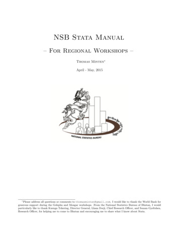
NSB Stata Manual– For Regional Workshops –Thomas Minten April - May, 2015 Please address all questions or comments to thomasminten@gmail.com. I would like to thank the World Bank forgenerous support during the Gelephu and Mongar workshops. From the National Statistics Bureau of Bhutan, I wouldparticularly like to thank Kuenga Tshering, Director General, Lham Dorji, Chief Research Officer, and Sonam Gyeltshen,Research Officer, for helping me to come to Bhutan and encouraging me to share what I know about Stata.
Information on WorkshopThrough the work of the National Statistics Bureau and many other government agencies, statisticalinformation is becoming more widely available in Bhutan. This offers the opportunity for Bhutanesegovernment employees to analyze and interpret data relevant to their decision-making. Yet many government officials lack the practical skills to analyze and present this data in an appropriate way. ThisStata Workshop is intended to help government officers to meaningfully make use of collected data. After this course, participants will be able to work with Stata and perform their own rudimentary analyses.In many government agencies and universities, Stata has become a standard program to analyze andpresent data, as it is both accessible and user friendly. This course will focus on using Stata to plan,carry out, and communicate analyses of real Bhutanese data sets. Rudimentary knowledge of statisticsis assumed. The workshop will be taught from a practical perspective. It will teach participants tobecome familiar with Stata, and in particular the course will teach participants the following:- To become familiar with Stata and its basic commands- To read any kind of data of public sources into Stata- To prepare data for analysis- To perform rudimentary analysis and statistical techniques- How to interpret the Stata output- How to present different types of data and insights in a meaningful wayThe Stata Workshop is specifically tailored to the needs of Bhutanese Statistical Officers and Researchers: The participants have the opportunity to use Bhutanese data sets such as the BLSS (BhutanLiving Standards Survey) 2012, or ADS (Annual Dzonkhag Survey) or data from the Statistical Yearbook. Using Bhutanese data in exercises during the workshop has the side-effect that participantswill become more familiar with the data available in Bhutan, and they learn interesting facts aboutBhutanese development along the way.The lecture notes include everything that is learned in the Stata workshop. The notes are stronglymodified material for the use during the workshop of National Statistics Bureau of Bhutan. I want tothank Andrea Linarello, Miguel Martinez, Paula Garda and Maria Paula Gerardino for the BGSE Statanotes on which this workshop notes are based. Yet, all remaining errors are my own. While readingthese notes, it is advantageous to try out the commands and new methods in Stata, and make the exercises that will be provided to you during the workshop. But most important is that you enjoy learning!Tashi Delek,Thomas1
Contents1 Introduction to Stata51.1The Stata environment . . . . . . . . . . . . . . . . . . . . . . . . . . . . . . . . . . . . .51.2Introducing commands . . . . . . . . . . . . . . . . . . . . . . . . . . . . . . . . . . . . .51.3Help files . . . . . . . . . . . . . . . . . . . . . . . . . . . . . . . . . . . . . . . . . . . .61.4Installing new commands . . . . . . . . . . . . . . . . . . . . . . . . . . . . . . . . . . .71.5Data import . . . . . . . . . . . . . . . . . . . . . . . . . . . . . . . . . . . . . . . . . . .71.6Describing the data . . . . . . . . . . . . . . . . . . . . . . . . . . . . . . . . . . . . . . .91.7Log files . . . . . . . . . . . . . . . . . . . . . . . . . . . . . . . . . . . . . . . . . . . . .101.8Do-files . . . . . . . . . . . . . . . . . . . . . . . . . . . . . . . . . . . . . . . . . . . . .101.9Commenting in do-files . . . . . . . . . . . . . . . . . . . . . . . . . . . . . . . . . . . . .112 Internet Resources and Data Import132.1Some useful internet resources on Stata . . . . . . . . . . . . . . . . . . . . . . . . . . .132.2Some useful Bhutanese data from the NSB. . . . . . . . . . . . . . . . . . . . . . . . .13National Statistics Bureau . . . . . . . . . . . . . . . . . . . . . . . . . . . . . . .13Some useful cross-country data from the internet . . . . . . . . . . . . . . . . . . . . . .142.3.1Penn World Table (http://pwt.econ.upenn.edu) . . . . . . . . . . . . . . . . . . .142.3.2Worldbank (http://data.worldbank.org) . . . . . . . . . . . . . . . . . . . . . . .162.3.3Bureau of Economic Analysis (http://www.bea.gov) . . . . . . . . . . . . . . . .182.3.4The Bureau of Labor Statistics (BLS) (www.bls.gov) . . . . . . . . . . . . . . . .182.2.12.33 Data Cleaning203.1General syntax in Stata . . . . . . . . . . . . . . . . . . . . . . . . . . . . . . . . . . . .203.2Generating new variables . . . . . . . . . . . . . . . . . . . . . . . . . . . . . . . . . . .203.3Dropping variables and observations . . . . . . . . . . . . . . . . . . . . . . . . . . . . .223.4Labeling and renaming existing variables . . . . . . . . . . . . . . . . . . . . . . . . . . .233.5Generate series of dummies out of a categorical variable . . . . . . . . . . . . . . . . . .243.6Recoding categorical variables . . . . . . . . . . . . . . . . . . . . . . . . . . . . . . . . .243.7Sorting . . . . . . . . . . . . . . . . . . . . . . . . . . . . . . . . . . . . . . . . . . . . . .253.8Other commands . . . . . . . . . . . . . . . . . . . . . . . . . . . . . . . . . . . . . . . .253.9Combining data sets . . . . . . . . . . . . . . . . . . . . . . . . . . . . . . . . . . . . . .263.10 Collapsing data sets . . . . . . . . . . . . . . . . . . . . . . . . . . . . . . . . . . . . . .274 Basic Statistical Routines and Tests284.1Descriptive Statistics . . . . . . . . . . . . . . . . . . . . . . . . . . . . . . . . . . . . . .284.2Saved Results . . . . . . . . . . . . . . . . . . . . . . . . . . . . . . . . . . . . . . . . . .302
4.3Correlations of Variables . . . . . . . . . . . . . . . . . . . . . . . . . . . . . . . . . . . .314.4T-Test . . . . . . . . . . . . . . . . . . . . . . . . . . . . . . . . . . . . . . . . . . . . . .314.5Cross-Tabulation and Chi-Square Test . . . . . . . . . . . . . . . . . . . . . . . . . . . .324.6Ordinary Least Squares (OLS) . . . . . . . . . . . . . . . . . . . . . . . . . . . . . . . .325 Time Series and Panel Data5.15.234Part I: Time series . . . . . . . . . . . . . . . . . . . . . . . . . . . . . . . . . . . . . . .345.1.1tsset - Declare data to be time-series data . . . . . . . . . . . . . . . . . . . . . .355.1.2Construct a Stata date variable from numerical components . . . . . . . . . . . .355.1.3Construct a Stata-date variable from scratch . . . . . . . . . . . . . . . . . . . .365.1.4Convert a string to a Stata-date variable . . . . . . . . . . . . . . . . . . . . . . .365.1.5Time series operators . . . . . . . . . . . . . . . . . . . . . . . . . . . . . . . . .375.1.6Example of a time series function: calculate autocorrelations . . . . . . . . . . .37Part II: Panel data . . . . . . . . . . . . . . . . . . . . . . . . . . . . . . . . . . . . . . .385.2.1The reshape-command . . . . . . . . . . . . . . . . . . . . . . . . . . . . . . . . .385.2.2xtset - Declare data to be panel data . . . . . . . . . . . . . . . . . . . . . . . . .396 Programming406.1Local Macros . . . . . . . . . . . . . . . . . . . . . . . . . . . . . . . . . . . . . . . . . .406.2Loops . . . . . . . . . . . . . . . . . . . . . . . . . . . . . . . . . . . . . . . . . . . . . .426.2.1The foreach-loop . . . . . . . . . . . . . . . . . . . . . . . . . . . . . . . . . . . .426.2.2The forvalues-loop . . . . . . . . . . . . . . . . . . . . . . . . . . . . . . . . . . .436.2.3The while-loop . . . . . . . . . . . . . . . . . . . . . . . . . . . . . . . . . . . . .43The if-command . . . . . . . . . . . . . . . . . . . . . . . . . . . . . . . . . . . . . . . .446.37 Presenting Results457.1Descriptive Tables . . . . . . . . . . . . . . . . . . . . . . . . . . . . . . . . . . . . . . .457.2Regression Tables . . . . . . . . . . . . . . . . . . . . . . . . . . . . . . . . . . . . . . . .467.3Graphs . . . . . . . . . . . . . . . . . . . . . . . . . . . . . . . . . . . . . . . . . . . . . .487.3.1Scatter plot . . . . . . . . . . . . . . . . . . . . . . . . . . . . . . . . . . . . . . .487.3.2Matrix of scatter plots . . . . . . . . . . . . . . . . . . . . . . . . . . . . . . . . .507.3.3Line plot . . . . . . . . . . . . . . . . . . . . . . . . . . . . . . . . . . . . . . . .507.3.4Plot a cumulative distribution function (cdf) . . . . . . . . . . . . . . . . . . . .517.3.5Histogram . . . . . . . . . . . . . . . . . . . . . . . . . . . . . . . . . . . . . . . .517.3.6The by option. . . . . . . . . . . . . . . . . . . . . . . . . . . . . . . . . . . . .517.3.7Other graphs . . . . . . . . . . . . . . . . . . . . . . . . . . . . . . . . . . . . . .527.3.8Combining graphs . . . . . . . . . . . . . . . . . . . . . . . . . . . . . . . . . . .527.3.9Producing nice graphs: titles, legends, notes, schemes, etc.523. . . . . . . . . . . .
7.3.10 Overview of options for graph layout . . . . . . . . . . . . . . . . . . . . . . . . .547.3.11 Templates for nice graphs . . . . . . . . . . . . . . . . . . . . . . . . . . . . . . .558 Advanced Topics8.18.257Advanced commands . . . . . . . . . . . . . . . . . . . . . . . . . . . . . . . . . . . . . .578.1.1The by-command in combination with n and N . . . . . . . . . . . . . . . . . .578.1.2collapse . . . . . . . . . . . . . . . . . . . . . . . . . . . . . . . . . . . . . . . . .598.1.3The preserve - restore commands . . . . . . . . . . . . . . . . . . . . . . . . . . .60Weights . . . . . . . . . . . . . . . . . . . . . . . . . . . . . . . . . . . . . . . . . . . . .604
1Introduction to StataThe first chapter is a general introduction to Stata. We will learn about the Stata environment, basicStata commands and help files. Also, we will learn how to read in different types of data into Stata,and how to describe and explore these data. In later chapters, we will look at these topics more indetail.1.1The Stata environmentOpen Stata 13. What do we see? Stata automatically displays 4 windows:1. Results: displays commands entered and corresponding output.2. Command: typing commands and executing them with enter key.3. Variables: displays the list of all the variables contained in the data set currently loaded. Youcan add a variable in the command window by clicking on the arrow left of its name.4. Properties: displays the properties of the data set and of the variables selected.There are other windows accessible through the corresponding icon of the toolbar: Data Editor (type edit in command balk and press enter): manual entry of data or manualcorrection of data (use cautiously; however you will be asked to confirm changes upon closing thewindow). Data Browser (browse) to view but not to edit data. Do-File Editor (doedit): to create do-files. Viewer (view): to open log files which are text file versions of the results window suitable forediting (also provides access to help files (help)).1.2Introducing commandsWhenever we want to do something in Stata, whether it is reading in data, or it is doing analyses, wehave to use commands. Commands can be issued in three ways:1. Menu: almost every command is included in the drop-down menus;- advantage: you don’t need to know the correct name and syntax of the respective command andyou get a pretty good overview on what you can do with Stata;- disadvantage: takes much more time than using the command line.5
2. Command line: good if you want to introduce your commands one by one;- advantage: doesn’t take much time;- disadvantage: you have to know the correct syntax (note: Stata is case-sensitive!).3. Do-file: collection of commands which can be executed together;- advantage: allows you to rerun a whole sequence of many commands with small changes, don’tneed to type in all of them manually, also a very good tool to “save” your work;- disadvantage: you have to know the correct syntax, more time intensive if you just want tocheck out one or two things.Important comment: For everything that is a bit longer than just one or two commands, creating ado-file is preferable! Almost every researcher uses do-files as the main way to run analyses in Stata.By default Stata works in the directory displayed on the bottom left of the screen (you can also typecd to see your working directory). It is possible to change the working directory by typing cd followedby the new path. In this way, any input (output) is read (written) in this path:cd "c:\Stata\Data"Example of three different ways to introduce commands: We want to use the data set work.dta.We need the command use filename [, clear] to get it into Stata. (The part of the commandin brackets [] is optional.)1. Menu: file open (or shortcut) select file work.dta (then you see the correct command spelledout in the results window and the variables included in the data set in the variables window)2. Command: Type in the following in the command line.cd "c:\Stata\Data"use work.dta, clear3. Do-file: Window Do-file editor New do-file (or shortcut doedit in command line) Typecd "c:\Stata\Data"use work.dta, clear Run (or Do).1.3Help filesStata is such an extensive program that it is impossible to know all the commands and their optionsby heart. If you can’t remember a particular command or the options available, use the help files. Helpfiles provide good information about all a command has to offer, and are used by Stata experts a lot.6
When you want to search for a keyword, e.g. the command use, you can use Stata to search for helptopics that contain that keyword. You can do this in two ways:1. typing in the command window search use or help use and press enter2. click “Help” “Stata Command” type “use”The help file for a command always contains: Title of command Syntax (the way to write it properly) Description (what does the command do) Options (what are the options doing) Examples (provide some fully worded out command examples)The findit command provides the broadest possible keyword search for Stata-related information. Itis equivalent to click Help, Search, Search all, then type “use”.1.4Installing new commandsThis findit command is also useful for finding code that is beyond the current installation of Stata.You can find this material by using the findit command and installing the code as a free user-writtencommand. It is easy to install provided you are connected to the Internet. The way you install suchcommands aressc install pkgname [, all replace]An example of a command that is not in the Stata 13 installation, but is often used by academicresearchers is outreg2. This command is used for a nice-looking output of regressions. If you areconnected to the internet, you can install it as follows:Typessc install outreg2The command will be installed, and this will usually take a short while. After it is finished, you canget information on this command by typinghelp outreg2.1.5Data importAfter getting somewhat familiar with the Stata environment, it’s now time to read in the data so wecan start doing analyses!There are several types of input file in Stata, the most common are: .raw for raw data, .dct for data plus7
variable names (dictionaries), .do for batch files containing Stata commands, .ado for Stata programs,and .log for log files. Data files in Stata format are given the extension .dta. These are created usingsave filename and read in with use filename.The following list gives info on how to read in data. Often, if you do real research, the data is notyet in Stata format (.dta format). For example the data you receive can come in .xls format, or .txtformat. Then you will have to import it yourself into Stata. It might be tempting to copy the datafrom Excel and paste it in the Stata Data Editor, but this is not the way to go! The data format maynot be conserved, so it is better to use one of the Stata commands to read in the data. If data is in .dta format already reading in is easy as we have seen before:cd "c:\Stata\Data"use work.dta, clear If the data is in text files (ASCII), or excel or csv format (where values are separated by tabsor commas), the best way is to open the file in Excel, and save it as a csv file, and then use theinsheet command:1. open the text, excel- or csv-file in Excel2. save it as csv-file (.csv extension) in Excel3. open Stata and enter commandinsheet using filename, clear [names]insheet can read in a text file in which there is one observation per line and the first line of thefile can contain the variable names (if that is the case, you should add the option names). Theoption clear should be used if you want to replace the current data in the memory. A free-format ASCII text file with space-, tab-, or comma-delimited data may be read with theinfile command. The missing-data indicator (.) may be used to specify that values are missing.The command must specify the variable names. Assuming mydata.raw contains numeric data,infile price mpg displacement using mydataIf some of the data are string variables without embedded spaces, they must be specified in thecommand:infile str3 country price mpg displacement using mydatawould read a three-letter country of origin code, followed by the numeric variables. The numberof observations will be determined from the available data. An other command that can be used to read in data is infix. Seehelp infixif you want to learn more about this command. They offer more options (for example if eachobservation spreads out over two lines).8
1.6Describing the dataNow that we know how to read in data, we can finally begin exploring data. If we start working with anew data set, it is important to get familiar with the data. You need to have a good idea of what youcan do with the data before you start doing analyses. Therefore, have a close look at the content, i.e.,what variables are in the data set, what values do these variables have, how many observations for each.The most useful commands that are used when looking for general information about data are: describe,summarize, and tabulate.First we read in the work.dta data set. describe [varlist] [, options] gives you some information about the name of thevariables, their storage type, their display format (with how many digits presented), and whetherthere are any labels for values or variablesExample: describe, all summarize [varlist] [, options] displays the number of observations per variable,mean, std. deviation, min and max valuesExample: summarizeor if you want extra details for each variablesummarize, detailor if you just want info on three variablessummarize age region stat, detail tabulate varname [,options] displays the number of observations per value of a variable, as well as the percentage shares and cumulative sharesExample: tabulate qualstabulate varname1 varname2 [,options] gives you a two-way table of the frequencies for two different variablesExample: tabulate ethnic qualsThere are many different options to the tabulate command. missing includes all the observations where the variable is missing. If you do not put this as an option, only non-missingobservations are counted. plot gives you a nice looking plot with your table, and sort displaysthe table in descending order of frequency. row or column let you define how percentages arecalculated in your table. Let’s try them out:tabulate ychildtabulate ychild, missingtabulate age, plot9
tabulate quals, sorttabulate ethnic qualstabulate ethnic quals, rowtabulate ethnic quals, column1.7Log filesYour actions and the results can only be traced back for a limited time in the results window. If youwant to ensure that you have a record of everything what you did, create a log file of your session.All output appearing in the Results window can be can be captured in a log file. The log file can besaved as a Stata formatted (SMCL) or as a text (ASCII) file.The necessary commands are as follows. To start the log file:log using filename [, options]To close the log file:log close.1.8Do-filesInstead of typing Stata commands directly into the command window and capturing all the output in alog file, it is also possible to create so-called do-files. A do-file is a text-file that contains a list of Statacommands (one for each line). When the do-file is executed, Stata processes all the commands that arelisted in the do-file. The main advantage of using do-files is that results can always be reproduced.Why is it better to use a do-file instead of just writing down all the commands in the command window?- Correction of errors and running again your code.- The analysis can be saved and the results can be replicated.- You can include comments (easier to organize your analysis).You should try to have a good routine to make do-files for everything you do in Stata. Let’s now makea do-file. The do-file editor can be opened by typingdoeditor click the do-file editor icon.Now there should be an editor with an empty do-file on the screen. Let’s type the following list ofcommands in the new do-file.clear allcd "c:\Stata\Data"use CPSsummarize wage10
To run a do-file click “Tools” (Do-file editor) and then choose “Do”. Alternatively you can click the“Do current file” icon (the one like a written sheet with a down arrow). It is also possible to run ado-file by typing do mydofile.do in the command line. But clicking the “Do current file” icon has theadvantage that you can select and run only a part of a do-file.By default, Stata output is sent to the screen. But you can save your output in a separate file, as wehave already seen. The log-file makes easier to review results by viewing this file using a text editor.The log-file can be created in the do-file and a useful convention is to give the log the same filename asthat for the do-file. Frequently, the following commands appear in the first lines of a do-file:The following commands will clear all the things Stata has in its memory, and opens the file you want,and let the do-file run even if it is very long.clear allset more offcd "c:\Stata\Data"use work.dtaIf you then want to capture the log, even as Stata closes and there is an error:capture log closeThen of course you want to save your logfile. The replace option permits the existing version of logfile.logto be rewritten. Without this option, Stata will refuse to open the log-file if there is already a file calledlogfile.log.log using logfile.log, replaceAnd at the end you might want to save your data and to close your log file.save mydata.dta, replacelog close.1.9Commenting in do-filesYou can add comments to a do-file, that will not be executed as Stata code. Comments have thepurpose to make the Stata code more readable and understandable. This is particularly important iftwo or more persons work on the same code. Lines defined as comments are ignored by Stata. Thereare three ways of defining parts of a do-file as a comment A line that begins with * is a comment In a line, everything that comes after a // is a comment Comments that go over more than one line are started with /* and stopped with */ For example,I could add comments do the do-file we just created.11
/*description:this is a very simple do-file with comments*/clear all // drops all variables*now we open the data setuse CPSsummarize wageAs you can see, the output that Stata produces from this do-file is the same as above. That is, Stataignores all the lines defined as comments. Again, the only purpose of comments is to make the do-filemore readable for the programmer. If you have a very long command, you can also break lines with///, and then continue in the next line.Quietly command: the quietly command suppresses the output of a command and it is not printedinto the log-file:quietly summarize wage12
2Internet Resources and Data ImportIn this chapter, it is discussed where you can find general information on Stata, and international andBhutanese data sets. We will also see many examples of how data are read into Stata.2.1Some useful internet resources on StataAn important rule about Stata is that almost any problems have been already solved by somebodyelse, and the answers are often put on the internet. Learn and practice how to search with google theanswer to your questions/problems. There are many pages with Stata tutorials online (search Statatutorial on google if you want alternative explanations to this m/links/video-tutorials/2.22.2.1Some useful Bhutanese data from the NSBNational Statistics BureauThe following Bhutanese data from the National Statistics Bureau is publicly available to everyone.Some of these files are in Excel format and therefore are easily importable into Stata. A problem withsome of the other data is that it is in pdf format, and this is almost impossible to import in Stata. Thebest strategy for you, if you want to work with this data that is in pdf format, is to ask the people atthe NSB to share the Excel data. Annual Dzongkhag Statistics: these statistics can be found on the website of NSB, and these include statistics on many areas including population, demographic statistics, health and nutrition,education, law enforcement, geography, elections, RGOB finances,. Population and Housing Census Data Consumer Price Index National Account Statistics Producer Price Index Statistical Year BookOn the NSB website, you also have the following big data sets. These are micro data, and so theyare very detailed, and are often on the individual or household level. You might need permission todownload these data sets.13
Bhutan Living Standard Survey 2007, Second Round Bhutan Multiple Indicator Survey 2010 Consumer Price Survey 2010 Health Facility Survey 2009 Labour Force Survey 2010 Population and Housing Census of Bhutan 2005 Renewable Natural Resources (RNR) Census 20092.3Some useful cross-country data from the internetHere we will see some examples of where to get economic data in international sources, and we willgo through these together. Usually, the data is not directly provided in the Stata .dta format on theinternet. Therefore, we will discuss at length how to import this data into Stata.2.3.1Penn World Table (http://pwt.econ.upenn.edu)The Penn World Table provides yearly data on GDP, consumption, exports, price indices, etc. for189 countries and territories. Data exists for some or all of the years between 1950-2010, the year ofreference 2005. (Latest update: 2013). The biggest advantage of the Penn World Table data is that thedata is denominated in a common set of prices in a common currency so that real quantity comparisonscan be made – both between countries and over time!Example: import population (POP) and GDP in constant 2005 prices (rgdpch) for Bhutan and Indiafrom 1950 to 2010 from the version of PWT version 7.1 from pwt.sas.upenn.eduData Download select countries Bhutan and India check variables rgdpch and POP select all years select comma-separated values (csv) click on “Send” copy the text, including the first line into notepad save the file as bhutanindia.csv file in your Stata folderImporting the data into Stata: Open Stata. Before you use the insheet command to import data youneed to check that bhutanindia.csv is actually in the current Stata directory. You can see what thecurrent Stata directory is by using cd. You can use the cd command to change directories.cdcd "c:\Stata\Data"14
In order to see the contents of the current directory typedirYou can show the contents of the data file you want to import by using the type command:type bhutanindia.csvNow you see the .csv-file on the screen. Notice the following things. 1) The first line gives the variablenames. The data only starts from line 2 on. 2) Missing values are represented by “na” (not available).(For example, between 1950 and 1969 the variable rgdpch is not available for Bhutan.)insheet using bhutanindia.csv, names clearThe names-option of the insheet command tells Stata that the variable names are stored in the firstline! The clear-option of the insheet command tells Stata to open a new data set from scratch.Now typedescribeYou can see that the variables country, countryisocode, and rgdpch are string variables. Some thingsto know about the variables in Stata: Case sensitivity: Stata is case sensitive. This means that female, Female or FEMALE are differentnames. The norm is to use lowercase. Variable names can be up to 32 characters long (A-Z; a-z;0-9; ). Some names such as in are reserved. * Asterisk: you can use the asterisk for variable names in commands. For example, describe c*displays information on the variables with names begining with the letter c. Storage type: Associated with each type of variable there is a storage type:– Nonnumeric data are recorded as strings, typically enclosed in double quotes such as “Bhutan”.They can be a combination of alphabetic and numeric characters. They are stored as str%.Two useful commands related with string variables are destring, which converts stringdata to integer data and tostring, which does the reverse.– Real variables: double (16 digits of accuracy) and float (about 7 digits of accuracy).– Integer variables: long (integers between -2,147,483,648 and 2,147,483,646), int (integersbetween -32,768 and 32,766) and byte (integers between -127 and 126).You can check which type of variables you have by typing in the command prompt: edit or browse.String variables are here printed in red font. That the country name is saved as a string variable isnatural. However, the GDP of a co
Stata Workshop is intended to help government o cers to meaningfully make use of collected data. Af-ter this course, participants will be able to work with Stata and perform their own rudimentary analyses. In many government agencies and universities, Stata has become a standard program to analyze and
