Transcription
An Introduction to Stata for HealthResearchersFifth EditionSVEND JUULDepartment of Public HealthAarhus UniversityAarhus, DenmarkMORTEN FRYDENBERGAarhus, Denmark A Stata Press PublicationStataCorp LLCCollege Station, Texas
Copyright c 2006, 2008, 2010, 2014, 2021 by StataCorp LLCAll rights reserved. First edition 2006Second edition 2008Third edition 2010Fourth edition 2014Fifth edition 2021Published by Stata Press, 4905 Lakeway Drive, College Station, Texas 77845Typeset in LATEX 2εPrinted in the United States of America10 9 8 7 6 5 4 3 2 1Print ISBN-10: 1-59718-315-6Print ISBN-13: 978-1-59718-315-4ePub ISBN-10: 1-59718-316-4ePub ISBN-13: 978-1-59718-316-1Mobi ISBN-10: 1-59718-317-2Mobi ISBN-13: 978-1-59718-317-8Library of Congress Control Number: 2021933404No part of this book may be reproduced, stored in a retrieval system, or transcribed, in any form orby any means—electronic, mechanical, photocopy, recording, or otherwise—without the prior writtenpermission of StataCorp LLC.Stata,,StataCorp LLC.Stata Press,Mata,,and NetCourse are registered trademarks ofStata and Stata Press are registered trademarks with the World Intellectual Property Organization of theUnited Nations.NetCourseNow is a trademark of StataCorp LLC.LATEX 2ε is a trademark of the American Mathematical Society.
ContentsList of tablesxiList of figuresxiiiPreface to the fifth editionxviiPreface to the first editionxixOnline supplementsxxiNotations in this bookxxiiiIThe basics11Getting started31.1Installing and updating Stata . . . . . . . . . . . . . . . . . . . . . . . .31.2Starting and exiting Stata . . . . . . . . . . . . . . . . . . . . . . . . . .71.3Windows in Stata . . . . . . . . . . . . . . . . . . . . . . . . . . . . . .91.4Issuing commands . . . . . . . . . . . . . . . . . . . . . . . . . . . . .151.5Managing output . . . . . . . . . . . . . . . . . . . . . . . . . . . . . .171.6Stata file types and names . . . . . . . . . . . . . . . . . . . . . . . . . .191.7Keyboard shortcuts . . . . . . . . . . . . . . . . . . . . . . . . . . . . .2123Getting help—and more232.1The help and search commands . . . . . . . . . . . . . . . . . . . . . . .232.2The complete Stata manuals . . . . . . . . . . . . . . . . . . . . . . . .272.3Other resources . . . . . . . . . . . . . . . . . . . . . . . . . . . . . . .28Command syntax313.1General syntax rules . . . . . . . . . . . . . . . . . . . . . . . . . . . .313.2Syntax diagrams . . . . . . . . . . . . . . . . . . . . . . . . . . . . . . .313.3Lists of variables and numbers . . . . . . . . . . . . . . . . . . . . . . .333.4Qualifiers . . . . . . . . . . . . . . . . . . . . . . . . . . . . . . . . . .34
Contentsvi3.5Weights . . . . . . . . . . . . . . . . . . . . . . . . . . . . . . . . . . .353.6Options . . . . . . . . . . . . . . . . . . . . . . . . . . . . . . . . . . .363.7Prefixes . . . . . . . . . . . . . . . . . . . . . . . . . . . . . . . . . . .373.8Other syntax elements . . . . . . . . . . . . . . . . . . . . . . . . . . . .373.9Version control . . . . . . . . . . . . . . . . . . . . . . . . . . . . . . .393.10Commands that influence program flow . . . . . . . . . . . . . . . . . .393.11Errors and error messages . . . . . . . . . . . . . . . . . . . . . . . . . .41IIData management434Variables454.1Numeric variables . . . . . . . . . . . . . . . . . . . . . . . . . . . . . .454.2Missing values . . . . . . . . . . . . . . . . . . . . . . . . . . . . . . .474.3Storage types and precision . . . . . . . . . . . . . . . . . . . . . . . . .494.4Date and time variables . . . . . . . . . . . . . . . . . . . . . . . . . . .514.5String variables . . . . . . . . . . . . . . . . . . . . . . . . . . . . . . .554.6Memory considerations . . . . . . . . . . . . . . . . . . . . . . . . . . .60567Getting data in and out of Stata615.1Opening and saving Stata data . . . . . . . . . . . . . . . . . . . . . . .615.2Entering data . . . . . . . . . . . . . . . . . . . . . . . . . . . . . . . .645.3Exchanging data with other software . . . . . . . . . . . . . . . . . . . .65Adding explanatory text to data696.1Variable and value labels . . . . . . . . . . . . . . . . . . . . . . . . . .696.2Dataset label and notes . . . . . . . . . . . . . . . . . . . . . . . . . . .72Calculations737.1generate and replace . . . . . . . . . . . . . . . . . . . . . . . . . . . .737.2Operators and functions in calculations . . . . . . . . . . . . . . . . . . .757.3The egen command . . . . . . . . . . . . . . . . . . . . . . . . . . . . .787.4Recoding variables . . . . . . . . . . . . . . . . . . . . . . . . . . . . .807.5Checking correctness of calculations . . . . . . . . . . . . . . . . . . . .817.6Giving numbers to observations . . . . . . . . . . . . . . . . . . . . . .82
Contentsvii8Commands affecting data structure858.1Selecting observations and variables . . . . . . . . . . . . . . . . . . . .858.2Renaming and reordering variables . . . . . . . . . . . . . . . . . . . . .868.3Sorting data . . . . . . . . . . . . . . . . . . . . . . . . . . . . . . . . .878.4Combining files . . . . . . . . . . . . . . . . . . . . . . . . . . . . . . .878.5Restructuring data . . . . . . . . . . . . . . . . . . . . . . . . . . . . . .929Taking good care of your data979.1Folders, filenames, variable names, and labels . . . . . . . . . . . . . . .989.2Data management . . . . . . . . . . . . . . . . . . . . . . . . . . . . . .1019.3Analysis . . . . . . . . . . . . . . . . . . . . . . . . . . . . . . . . . . .1129.4Protect your data . . . . . . . . . . . . . . . . . . . . . . . . . . . . . .113III Analysis11510Description and simple analysis11710.1Overview of a dataset . . . . . . . . . . . . . . . . . . . . . . . . . . . .11710.2Listing observations . . . . . . . . . . . . . . . . . . . . . . . . . . . . .12010.3Simple tables for categorical variables . . . . . . . . . . . . . . . . . . .12210.4Analyzing binary variables . . . . . . . . . . . . . . . . . . . . . . . . .12710.5Analyzing continuous variables . . . . . . . . . . . . . . . . . . . . . . .13210.6Estimating confidence intervals . . . . . . . . . . . . . . . . . . . . . . .14110.7Immediate commands . . . . . . . . . . . . . . . . . . . . . . . . . . . .14211Regression analysis14511.1Linear regression . . . . . . . . . . . . . . . . . . . . . . . . . . . . . .14511.2Regression postestimation . . . . . . . . . . . . . . . . . . . . . . . . .14811.3Categorical predictors—factor variables . . . . . . . . . . . . . . . . . .15011.4Interactions in regression models . . . . . . . . . . . . . . . . . . . . . .15611.5Logistic regression . . . . . . . . . . . . . . . . . . . . . . . . . . . . .16311.6Other regression models . . . . . . . . . . . . . . . . . . . . . . . . . .16911.7Nonindependent observations . . . . . . . . . . . . . . . . . . . . . . . .16911.8Bootstrapping . . . . . . . . . . . . . . . . . . . . . . . . . . . . . . . .171
Contentsviii12131415Time-to-event data17512.1Setting the time scale and event: The stset command . . . . . . . . . . .17712.2The Kaplan–Meier survival function . . . . . . . . . . . . . . . . . . . .17912.3Tabulating rates . . . . . . . . . . . . . . . . . . . . . . . . . . . . . . .18212.4Cox proportional hazards regression . . . . . . . . . . . . . . . . . . . .18512.5Preparing data for advanced survival analyses . . . . . . . . . . . . . . .19112.6Advanced survival modeling . . . . . . . . . . . . . . . . . . . . . . . .19312.7Poisson regression . . . . . . . . . . . . . . . . . . . . . . . . . . . . .197Power, precision, and sample-size analysis20113.1Power analysis . . . . . . . . . . . . . . . . . . . . . . . . . . . . . . .20113.2Precision analysis . . . . . . . . . . . . . . . . . . . . . . . . . . . . . .20513.3Power by simulation—A superiority study . . . . . . . . . . . . . . . . .206Measurement and diagnosis20914.1Comparing two measurements . . . . . . . . . . . . . . . . . . . . . . .20914.2Reproducibility of measurements . . . . . . . . . . . . . . . . . . . . . .21314.3Using tests for diagnosis . . . . . . . . . . . . . . . . . . . . . . . . . .216Miscellaneous22515.1Random samples, simulations . . . . . . . . . . . . . . . . . . . . . . .22515.2Working with diagnoses . . . . . . . . . . . . . . . . . . . . . . . . . . .22715.3Preparing tables for publication . . . . . . . . . . . . . . . . . . . . . . .23615.4Including graphs in Word and PDF files . . . . . . . . . . . . . . . . . .24715.5Profile.do changing the ado-path . . . . . . . . . . . . . . . . . . . . . .25015.6Unicode and ASCII encoding of characters . . . . . . . . . . . . . . . .25115.7Other analyses . . . . . . . . . . . . . . . . . . . . . . . . . . . . . . . .251IV Graphs25316Graphs25516.1Anatomy of a graph . . . . . . . . . . . . . . . . . . . . . . . . . . . . .25616.2Anatomy of graph commands . . . . . . . . . . . . . . . . . . . . . . . .25716.3Graph size . . . . . . . . . . . . . . . . . . . . . . . . . . . . . . . . . .258
Contentsix16.4Schemes . . . . . . . . . . . . . . . . . . . . . . . . . . . . . . . . . . .26116.5Graph options: Axes . . . . . . . . . . . . . . . . . . . . . . . . . . . .26316.6Graph options: Text elements . . . . . . . . . . . . . . . . . . . . . . . .26816.7Plot options: Markers, lines, etc. . . . . . . . . . . . . . . . . . . . . . .27216.8Histograms and other distribution graphs . . . . . . . . . . . . . . . . . .27716.9Twoway graphs: scatterplots and line plots . . . . . . . . . . . . . . . . .28116.10 Bar graphs . . . . . . . . . . . . . . . . . . . . . . . . . . . . . . . . . .29116.11 By-graphs and combined graphs . . . . . . . . . . . . . . . . . . . . . .29716.12 Saving and exporting graphs . . . . . . . . . . . . . . . . . . . . . . . .299VAdvanced topics30317Advanced topics30517.1Using stored results . . . . . . . . . . . . . . . . . . . . . . . . . . . . .30517.2Macros and scalars . . . . . . . . . . . . . . . . . . . . . . . . . . . . .31017.3Some useful commands . . . . . . . . . . . . . . . . . . . . . . . . . . .31317.4Programs . . . . . . . . . . . . . . . . . . . . . . . . . . . . . . . . . .31717.5Debugging programs and complex commands . . . . . . . . . . . . . . .321References323Author index325Subject index327
Preface to the fifth editionThis fifth edition updates the fourth edition to reflect the changes in Stata 14, released in 2015;Stata 15, released in 2017; Stata 16, released in 2019; and Stata 17, released in 2021.Since the fourth edition of the book, many nice things have happened with Stata, and manyof these changes are also reflected in the book. In several ways, Stata has become more userfriendly, for example, with an improved Do-file Editor.Stata now has commands for working with both the 9th and the 10th releases of the International Classification of Diseases, and we have included them in the book. We also included achapter on the much-improved commands for power, precision, and sample-size analysis. Withrelease 14, Stata introduced Unicode, giving the opportunity to use a wealth of characters beyond the Latin alphabet, and the consequences of that affect several sections in the book. Withrelease 17, Stata introduced tools to tailor publication-ready tables, and we wrote an introduction to these tools. Finally, we made a complete revision of the important (we think) chapter 9,Taking good care of your data.This is an introductory book aimed at people working in health research, and we had to makeseveral decisions about what to include and what to omit. If you miss something that is notdescribed in the book, it does not necessarily mean that Stata cannot do it. Use the helpcommand and the PDF manuals to learn more.During the process, Bill Rising and Kristin MacDonald at StataCorp gave several useful suggestions to improve the quality of the book, and Lisa Gilmore coordinated everything.User reactions are welcome and can be good inspiration for further improvements, so pleasefeel free to send comments to sj@ph.au.dk or mfstat@mollerfryd.dk.Aarhus, DenmarkJuly 2021Svend Juul and Morten Frydenberg
3 Command syntax3.1General syntax rulesStata’s language rules are described in detail in [U] 11 Language syntax; to get there, type. help languageStata is case sensitive, and all official Stata command names are lowercase. list is a validcommand, but List is not. Variable names may include lowercase and uppercase letters, butsex and Sex are two different variable names. Throughout this book, we use lowercase variablenames.Variable names can have up to 32 characters, but Stata often abbreviates long variable names inoutput, so we recommend avoiding more than, say, 10 characters. Numbers (0–9), letters (A–Z,a–z, and any Unicode letter), and (underscore) are valid characters in variable names. Namesmust start with a letter and can contain an underscore, but starting with an underscore shouldbe avoided because many Stata-generated temporary variables begin with an underscore. Thefollowing are valid variable names:a q17 q 17 pregnant sex3.2Syntax diagramsA syntax diagram is a formal description of the elements in a Stata command. The notation usedis described in [R] Intro, which you will find in the beginning of the Base Reference Manual[R]. The general syntax of typical Stata commands can be written like this: prefix: command varlistifinweight, optionsFor example, the syntax for summarize is summarize varlistifinweight, eparator(#)display optionsdisplay additional statisticssuppress the display; calculate only the mean; programmer’s optionuse variable’s display formatdraw separator line after every # variables; default is separator(5)control spacing, line width, and base and empty cells31
Chapter 3 Command syntax32Find a more detailed description of the syntax of summarize by typinghelp summarize Thin square brackets,, mean that the item is optional, so the only mandatory part of thesummarize command is the command name itself. Square brackets may also be part of thesyntax, in which case they are shown in the typewriter font, as in.tab2 case ctrl [fweight pop] Curly brackets,, mean that you must specify one of the options but not both options, as in numlabel lblname-list , add removeHere you must specify either add or remove.Command and option names can be abbreviated; in the syntax diagram, underlining showsthe minimum abbreviation. We use few abbreviations. Although they make commands fasterto write, they make them more difficult to read. Table 3.1 shows some example summarizecommands:Table 3.1. Example summarize commandsprefixby tionsCommentsall: all variablessummarizeAll variablessumAbbreviatedsummarizesex ageTwo variablessummarizesex-weightVariable rangesummarizepro*All variables startingwith prosummarize*ro*All variablescontaining rosummarize?ro?5-letter variables; ro as3rd and 4th characterssummarizeageif sex 1Males onlysummarizebmiin 1/10First 10 observationssummarizebmi[fweight n]Weighted e table for eachsex; data must besorted first, detailOption: detail
3.3 Lists of variables and numbers3.333Lists of variables and numbersVariable listsA variable list (varlist) defines one or more variables to be processed. Here are some examples:(nothing)Sometimes means the same as allallAll variables in the datasetsex age pregnantThree variablespregnant sex-weightpregnant and the consecutive variables from sex to weightpro*All variables starting with pro*ro*All variables containing ro?ro?five-letter variables with ro as third and fourth charactersWhen generating new variables, you can refer to the 17 variables q1, q2, . . . , q17 as q1-q17.When referring to existing variables q1-q17, you will get q1, q17, and the variables that comebetween them in the dataset, which are not necessarily q2, q3, . . . , q16. summarize anddescribe are useful commands to see the ordering of variables in the dataset.In commands that have a dependent variable, it is listed first in the variable list:. oneway bmi sexbmi is the dependent variable. regress bmi sex agebmi is the dependent variable. scatter weight heightScatterplot, weight is the y axis. tab2 expos caseThe first variable defines the rowsNumeric listsA numeric list (numlist) is a list of numbers with some shorthand possibilities:1(3)111(1)4 4.5(0.5)64 3 2 7(-1)11/54/2 7/1meansmeansmeansmeansmeans114144232373232104 4.5 5 5.5 67 6 5 4 3 2 14 57 6 5 4 3 2 1Numeric lists have many uses; for example, they can display person-time and incidence rates in 0.5-year intervals up to 5 years:. stptime, at(0(0.5)5) by(drug) show a graph with y-axis labels at 0 10 20 30 40:. scatter mpg weight, ylabel(0(10)40) generate age groups 0–4, 5–14, 15–24, . . . , 75–84, 85 :. egen agegrp cut(age), at(0 5(10)85 200)
Chapter 3 Command syntax34Numeric rangesNumeric lists should not be confused with numeric ranges. The following are ranges:1. list in 1/10. recode age (45/max 3)(25/45 2)(0/25 1), generate(agegr)3.4QualifiersQualifiers are common to many commands, while most options are specific to one command ora few commands.The if qualifierThe if qualifier is used with logical expressions to select the observations to which a commandapplies. Here are a few examples (sex has the value 1 for males):. summarize age if sex 1Males only. summarize age if sex! 1Males excluded. list id age if age 25Young only. replace npreg . if sex 1set npreg to missing for males. list sex age weight if sex 1 & age 25Young males only. keep if sex 1 age 25Males or young. keep if !(sex 1 age 25)All othersTwo types of operators are used in logical expressions, as shown in table 3.2.2Table 3.2. Operators in logical expressionsRelational operators ! Greater thanLess thanGreater than or equal toLess than or equal toEqualNot equalLogical operators! Not& And OrThe double equal sign ( ) in relational expressions has a meaning different from that of theassignment equal sign, as in. generate bmi weight/(height 2)1. You may wonder why we chose to let the recode command start with the highest values. See an explanation insection 7.4.2. Previously, the tilde ( ) was used for “Not”, and it still works, but it is seldom used.
3.5 Weights35Logical expressions are evaluated to be true or false. A value of 0 means false, and any othervalue, including missing values, means true. Technically, missing values are large positivenumbers and are evaluated as such in logical expressions. This issue is described in more detailin section 4.2.With complex logical expressions, use parentheses to control the order of evaluation:.list if ((sex 1 & wt 90) (sex 2 & wt 80)) & ! missing(wt)Omitting the parentheses might give a different selection, but the outcome may be difficult topredict. Use parentheses to make the syntax transparent to yourself; then it will work correctly.A possibly more transparent way to handle complex selections is to generate a help variable(heavy):. generate heavy 0Initialize help variable (heavy). replace heavy 1 if sex 1 & wt 90Include males 90 kg. replace heavy 1 if sex 2 & wt 80Include females 80 kg. replace heavy . if missing(wt)Do not include if wt is missing. list if heavy 1These are the heavy onesThe in qualifierThe in qualifier is used to select the observations to which a command applies. It is especiallyuseful for listing or displaying a subset of observations. Below are three examples:. list sex age weight in 2323rd observation. list in 1/10All variables; observations 1–10. browse sex-weight in -5/-1See last 5 observations in the Data BrowserThe last observation is identified by -1, and -5/-1 means the last five observations. Note thatthe sort order of the dataset may change, so you should not rely on the observation number toidentify a specific observation.3.5WeightsWeighting observationsWeights can be used to multiply observations when the input is tabular. Suppose that you seethe following table in a paper and want to analyze it l44130
Chapter 3 Command syntax36The input command (see section 5.2) lets you enter the tabular data directly:input1 11 00 10 0endexpos case pop213023100Now you can analyze the data by weighting with pop:.tab2 expos case [fweight pop], chi2logistic case expos [fweight pop]The square brackets around the weight expression are shown in typewriter font. They are partof the syntax; here they do not mean optional.fweight indicates frequency weighting. For information about other types of weighting, see.3.6help weightOptionsOptions are specific to a command, and you must use the help command or look in the PDFdocumentation to see the available options. Options come last in the command, and they arepreceded by a comma. Usually, there is no more than one comma per command, but complexgraph commands may include more; see chapter 16.The nolabel option is common to many commands. If value labels have been assigned to avariable, Stata usually displays the value label rather than the code in tables and listings. Thenolabel option lets you see the code instead of the label:.tab1 race- tabulation of 913.7635.4550.7964.55100.00Total189100.00tab1 race, nolabel- tabulation of .7964.55100.00Total189100.00
3.8 Other syntax elements3.737PrefixesOnly the by varlist: prefix is shown here, but in later chapters, we will illustrate others, forexample, quietly and statsby.The by varlist: prefixThe by varlist: prefix makes a command perform calculations or display results for strata of thedata. Data must be sorted by the stratification variables. The following commands lead to twosummarize tables, one for each sex:. sort sex. by sex: summarize age height weightThere are two ways to produce the same results with one command:. bysort sex: summarize age height weight. by sex, sort: summarize age height weight3.8Other syntax elementsText strings with quotesStata uses double quotes around text strings. This applies to filenames, file paths, and labels, asshown here:. label define sex 1 "male" 2 "female" 9 "sex unknown". use " /Documents/ishr5/lbw1.dta"Actually, quotes are not needed around text strings without spaces, but in this book, we mostoften use them to improve readability. The above commands could be written. label define sex 1 male 2 female 9 "sex unknown". use /Documents/ishr5/lbw1.dtaCommentsThe following are interpreted as comments, so you can include short explanations in do-filesand ado-files: Lines beginning with *. Text following //. If // are not the first characters in the line, they must be preceded bya space to work properly.Comments make your do-files more readable; Stata does not care what you write:. * /ado/personal/profile.do executes when opening Stata. // /ado/personal/profile.do executes when opening Stata. summarize bmi, detail// Body mass index
11 Regression analysisThis chapter describes the fundamentals of linear regression and logistic regression. However,many other regression models are available in Stata. Chapter 12 discusses Poisson regressionand Cox regression, and the general principles apply to them, too.We will not go into details of how to analyze data by regression models, but instead, we willfocus on some of the features in Stata: working with categorical explanatory variables, testinghypotheses, and using Stata’s postestimation facilities.Stepwise selection procedures are available in Stata, but they will generally lead to invalid estimates, confidence intervals, and p-values. Therefore, we will not describe them. Find a discussion of the problems at wise-regressionproblems/, What are some of the problems with stepwise regression?A regression model expresses the dependency of one variable (the response, outcome, or dependent variable) on one or more other variables (predictors, regressors, or independent variables).Short introductions to regression models can be found in many standard textbooks, such asKirkwood and Sterne (2003). If you want to apply more than the simplest regression models,you should consult books dedicated to the subject, such as Vittinghoff et al. (2012) and Hosmer,Lemeshow, and Sturdivant (2013).11.1Linear regressionWe are going to use the lbw.dta dataset but with added numerical labels; see section 10.1:. cd " /Documents/ishr5". use lbw1.dta(Hosmer and Lemeshow data - with labels).codebook, compactVariableObs 92261452503131164990145LabelIdentification codeBirthweight 2500gAge of motherLast prepregnancy weight (lb)RaceSmoked during pregnancyPremature labor history (count)Has history of hypertensionPresence, uterine irritabilityNumber of visits to physician du.Birthweight (grams)
Chapter 11 Regression analysis146We will start by looking at a simple linear regression model, which in Stata is fit using theregress command.1 Let us consider the modelbwt β0 β1 lwt errorHere bwt (birthweight in grams) is the dependent variable, and lwt (weight at last menstrualperiod in lb) is the predictor. error is the unexplained random variation; it is assumed normalwith mean zero and standard deviation σ. The estimates for β0 , β1 , and σ are easily found withthe regress command:. regress bwt bwtCoefficientStd. .37Number of obsF(1, 187)Prob FR-squaredAdj R-squaredRoot MSE 1896.690.01050.03450.0294718.24P t [95% conf. 8The estimate for β0 (2369.184) is found in the cons line, and the estimate for β1 (4.429993)is found in the lwt line. Confidence intervals for β0 and β1 are found in the two rightmostcolumns.The estimated relationship ismean bwt 2369.2 4.43 lwtA weight difference of 10 lb between two mothers corresponds to an expected difference inbirthweight of 44.3 grams; the 95% confidence interval is [10.5, 78.1]. Under the model, thatis, assuming linearity, the slope is significantly different from 0 (t 2.59; p 0.010). consis the constant or intercept, that is, the predicted outcome when all predictors are 0. Hereit is the predicted birthweight (2,369 grams) for a child whose mother weighed 0 lb. Naïveextrapolations outside the observed ranges of the predictors obviously can lead to nonsense.The estimated standard deviation of the error term, σ, is displayed in the upper-right block ofoutput as Root MSE; here it is 718.24. From σ, we can express the variation around the estimated regression line as a 95% prediction interval using 1.96·σ, here 1408 grams. Theregress command does not calculate the confidence interval around σ, but an unofficial program, cisd, does it for you. You can download the program by typing. ssc install cisdcisd is a postestimation command (see section 11.2), and it must be preceded by a regresscommand. Here we run it quietly because we have already seen the regress output:. quietly regress bwt lwt1. The regress command assumes that the precise value is observed. If you know only that the value lies within aninterval, that is, you have interval-censored data, you can use intreg.
11.1 Linear regression.147cisdSD(error): 718.2354995% CI: ( 652.23371 ; 799.21579 )In figure 11.1, a scatterplot with a regression line illustrates the association. You can find ado-file with the full graph command (gph fig11 1.do) at this book’s website, but here weshow the minimum graph command:.twoway (scatter bwt lwt) (lfit bwt lwt)Birthweight (grams)5000400030002000100050100150200250Last prepregnancy weight (lb)Figure 11.1. Scatterplot with a regression lineWe can fit a multiple regression model, that is, a model involving more than one predictor:bwt β0 β1 lwt β2 age error.regress bwt lwt ageSourceSSdfMSNumber of obsF(2, 186)Prob FR-squaredAdj R-squaredRoot ntStd. err.tP t 400.797.410.0170.4290.000lwtagecons 1893.650.02790.03780.0274718.95[95% conf. 2806.63From this, we can find the estimated relationship:mean bwt 2216.2 4.18 lwt 7.97 ageThe interpretation is that for each pound of maternal prepregnancy weight, the mean birthweightincreased by 4.18 grams when adjusted for maternal age.
Chapter 11 Regression analysis14811.2Regression postestimationOne of the nice features in Stata is that the default output from a regression analysis is limited to the most essential information, but afterward, it is possible to supplement an analysiswith additional information, such as calculating diagnostics (residuals, leverages, etc.), testingspecific hypotheses, displaying variance inflation factors, and displaying correlations betweenestimates. This is done with postestimation commands, and we will show some examples. Readabout postestimation commands in general by typing. help estimationand about specific commands by typing. help regress postestimationOne of the assumptions behind the regression model above is that the error term should followa normal distribution. This is validated by making a Q–Q plot or a histogram of the residuals.To do this, we need a new variable containing the residuals.2 This is easily generated by typing. quietly: regress bwt lwt age. predict rbwt if e(sample), residualThe predict command will generate a new variable, rbwt, containing the residuals. We ranthe regress command quietly because we had already recorded the output
Stata's language rules are described in detail in [U] 11 Language syntax; to get there, type . help language Stata is case sensitive, and all official Stata command names are lowercase. list is a valid