Transcription
19. Excel graphing instructions Page 1 of 3619. MS Excel dataand graphinginstructions Lawrence W. Braile,ProfessorDepartment of Earth andAtmospheric SciencesPurdue UniversityWest Lafayette, IndianaSheryl J. Braile, TeacherHappy Hollow SchoolWest Lafayette, IndianaFebruary 4, 2002Objective: This module provides instructions for using the MS Excel program to save,organize and graph data that are derived from SeisVolE analysis of earthquake andvolcano activity. Four main types of graphs are illustrated: histograms (or bar graphs),X-Y scatter plots, “event” plots, and bubble plots. Examples using data from SeisVolEanalyses and exploration are provided.Information: Microsoft Excel has become a standard spreadsheet program for storingdata sets and producing graphs. Excel is flexible, has many capabilities, and can be used Copyright 2001. L. Braile and S. Braile. Permission granted for reproduction for non-commercialpurposes.Seismic/Eruption Teaching Modules:19 - 1 -
19. Excel graphing instructions Page 2 of 36to generate effective and high-quality graphs (usually referred to as “charts” in Excel).Data and graphs produced in Excel are also easily printed or exported to word processingprograms such as Microsoft Word. The instructions below illustrate how to generate 4types of graphs (histogram, scatter plot, event plot, and bubble plot) that are useful fordisplaying earthquake data. These graphs can provide analysis and insight in addition tothat provided by viewing seismicity data on maps. For less-experienced Excel users,working through the instructions will illustrate many of the standard features andprocesses used in Excel and make it possible to perform many other tasks that arepossible with the program. In the instructions below, many of the steps are illustrated bya portion of a screen image, an image of the appropriate dialog box that appears in Excel,or a full screen image. Graphs should always be labeled so that the reader can clearlyunderstand the characteristics of the data that are being plotted. Graph axes should belabeled to indicate the measurement that is being plotted and the units (kilometers,seconds, years, percentage, number of occurrences, meters/second, kilograms, magnitude,etc.; appropriate abbreviations, such as km for kilometers or s for seconds can be used) ofthe observed values. A graph title (or caption) can be used to further describe the limitson the data and the data source.Graphing “by hand” is a significant skill that should be included in one’s experienceswith graphing. Graphing data with pencil and paper can produces quick, exploratoryresults and improves understanding of graphs, data and the interpretation of graphs.Graphing by hand is easily accomplished using standard, commercial graph paper.Additionally, some templates for some the graph types that are described here areprovided for use in “graphing by hand”. The first time (or more) that one uses aparticular graph type (such as histogram, X-Y scatter plot, X-Y plot with a logarithmicscale), an effective procedure is to graph the data by hand and then on the computer.The following sections provide instructions and examples for creating graphs usingExcel.1. Histogram (Bar or Column Graph) Plot: The histogram is a veryuseful graph for statistical data and summary information consisting of a relatively few(less than about 20-30) values. The X-axis values are often sequential but do not need tobe. They can be arbitrary classes or categories. The Y-axis values are often the numberof occurrences within each category. To create a histogram plot using Excel:a. Open Excel; a spreadsheet appears (or, from the File menu, select New).b. Enter data in columns (click on first cell in column to start, type number, hitenter, repeat). Enter data for additional column. For the histogram (or bargraph) plot, it is most convenient to have the first column be a list of non-Seismic/Eruption Teaching Modules:19 - 2 -
19. Excel graphing instructions Page 3 of 36numeric entries that describe the order of the data to be displayed in thehistogram. For example, for an aftershock sequence, the following data weredetermined (magnitude and time sort using SeisVolE for a small area in theAleutian Islands; the data are for the aftershocks of the Rat Island earthquake,M8.7, February 3, 1965; column A is the month in 1965; column B is thenumber of earthquakes in the selected area of magnitude greater than or equalto 5 during that month, from the counter on the SeisVolE screen):c. Select (highlight using the mouse, as shown above) the cells containing datathat you wish to plot. Click on the Chart Wizard icon at the top of the screen(the Chart Wizard icon looks like a color 3D histogram):d. Select the Column chart. Click Next. A dialog box with a graph previewwill appear. Click Next. Enter graph (chart) title, X-axis title and Y-axis title.Click Next. Click Finish.Seismic/Eruption Teaching Modules:19 - 3 -
19. Excel graphing instructions Page 4 of 36e. Enlarge the graph on the screen by clicking on the chart area, to select thechart, and dragging one or more of the small black squares along the rectanglethat surround the graph. To change the color of the bars in the histogram plot,double-click on one of the bars and select the color that you want. In thedialog box shown below, the color red has been selected for the bars.A view of the screen for the spreadsheet and histogram plot is shown below. TheSeismic/Eruption Teaching Modules:19 - 4 -
19. Excel graphing instructions Page 5 of 36graph is selected so the small black squares are visible. When selected, the graphwindow can be enlarged (drag one or more of the squares), printed, or copied andpasted (using the Edit menu) to another document such as Microsoft Word.To adjust the font size and type for the axis labels and titles, double-click on theitem that you wish to modify and make changes in the dialog box that appears.Select the font, font style and font size desired. For example, by double-clickingon an axis, the following dialog box is displayed. By selecting the Font option,the desired font type, font style and font size can be selected.Seismic/Eruption Teaching Modules:19 - 5 -
19. Excel graphing instructions Page 6 of 36To add the data value numbers (optional) at the top of each bar in the histogram,double-click on one of the histogram bars, select Data Labels in the resultingdialog box and click on Show Value.f. Save the spreadsheet and graph with the Save As command under File; enteran appropriate file name.g. You can print the spreadsheet page or the graph only (select the graph andSeismic/Eruption Teaching Modules:19 - 6 -
19. Excel graphing instructions Page 7 of 36then select print), or copy and paste to another document. An example of ahistogram graph is shown in Figure 19.1 (an additional example is containedin the Frequency-Magnitude instructions, Kuriles and Kamchatka area):Number of Earthquakes M5 2502361965 Rat IslandsAftershock Sequence20015010050442614117526850Feb Mar Apr May JunJul Aug Sep Oct Nov DecMonthFigure 19.1. Number of earthquakes of magnitude 5 and greater per month in the 1965Rat Islands (Aleutians) main shock/aftershock sequence. The main shock was amagnitude 8.7 event on February 3, 1965.A template for making histogram plots by hand is provided in Figure 19.2. The numberof columns is limited to 10 or less in this template. Similarly, the there are 10 amplitudetic marks on the Y axis. Axis labels (values on or between the tic marks) and adescription of the X and Y data must be added. The columns should be drawn in thespace between the X-axis tic marks, similar to those shown in the Excel histogram inFigure 19.1.Seismic/Eruption Teaching Modules:19 - 7 -
19. Excel graphing instructions Page 8 of 36Figure 19.2. Template for making a histogram by “plotting by hand”.Seismic/Eruption Teaching Modules:19 - 8 -
19. Excel graphing instructions Page 9 of 362. X-Y Scatter Plot: The X-Y scatter graph is used to plot points on a graphand examine the correlation between the X and Y variables (measurements) or thechange in the Y values as the X values increase. The description of X (for thehorizontal axis) and Y (for the vertical axis) is common usage, although the X andY variable represent measurements or observations. For example, the X variableis often time or distance and the Y variable is often an amplitude of a measuredquantity. The X values do not have to be sequential (increasing or decreasing),but if they are, it is common to connect the points on the graph with a line. Tocreate an X-Y scatter plot in Excel:a. To plot an X-Y scatter plot (x and y coordinates; plot with symbols, lines orsymbols and lines) in Excel, open Excel, and enter data as explained above.Enter the x coordinates in the first (A) column and the y coordinates in thesecond (B) column. Select the cells containing the data and click the ChartWizard icon. An example of some data entered into an Excel spreadsheet foran X-Y scatter plot is given below. The values are Frequency-Magnitude datafor the Kuriles and Kamchatka area obtained by using the earthquake counterin SeisVolE.Col. AMagnitude, MCol. BNumber of events, / Mb. Select the XY (Scatter) graph. Click Next and a dialog box with a preview ofthe graph will appear. Click Next and enter the graph title and titles for the Xand Y axes. Click Next and then Finish. Adjust font size and type by doubleclicking on the appropriate axis or label and modifying the information in theSeismic/Eruption Teaching Modules:19 - 9 -
19. Excel graphing instructions Page 10 of 36dialog box. Modify the symbol by double-clicking on a symbol andmodifying the information in the dialog box.To change the Y axis to a logarithmic (log) scale, double-click on the Y axis,select Scale and click on Logarithmic Scale. To turn on the plotting of minortick marks (on a logarithmic scale, 8 tick marks show the positions ofirregularly-spaced positions along the axis corresponding to tenths of themajor tick separation; for example, for the axis segment from 10 to 100, theminor tick marks will show the locations corresponding to 20, 30, 40, 50, 60,70, 80, and 90), double-click on the Y-axis and select Outside under theMinor Tick Mark area of the Patterns section of the dialog box.Seismic/Eruption Teaching Modules:19 - 10 -
19. Excel graphing instructions Page 11 of 36c. Save the spreadsheet and graph with the Save As command under the Filemenu. To make changes in the graph titles (main title and X- and Y-axis titles),select the graph with the mouse. Small black squares will appear on therectangular line that surrounds the graph and the word Chart will appear in thepull-down menu line. From the Chart menu, select Chart Options A dialogbox will appear which you can use to make changes in the titles as well as modifyor add some other features of the graph.d. You can print the spreadsheet page or the graph only (select the graph and thenselect print), or copy and paste to another document. An example of a FrequencyMagnitude plot, with logarithmic Y axis, for the Kuriles and Kamchatka data isshown in Figure 19.3. Notice that the points define an almost perfect straight lineon the frequency-magnitude plot with the logarithmic Y (frequency of events)axis plot. This relationship (sometimes called the Gutenberg-Richter relationshipafter the two seismologists who first described it) is an almost-universalcharacteristic of seismicity data for nearly all areas and time periods.Seismic/Eruption Teaching Modules:19 - 11 -
19. Excel graphing instructions Page 12 of 36Earthquakes in 41 Years M 10000Kuriles and KamchatkaEarthquakes 1960-200010001001014567Magnitude, M89Figure 19.3. Frequency-magnitude plot for the Kuriles and Kamchatka region. Alogarithmic Y-axis (frequency of events) is used.The same frequency-magnitude data plotted on a bar graph (or histogram) with a linear Yaxis (Figure 19.4) illustrates the rapid decrease in the number of events that occur in agiven region with each increase in magnitude. In general, for each increase of onemagnitude unit, there are about one-tenth as many earthquakes. Because some smallmagnitude events may not be detected, and because, for short time periods, the number oflarge earthquakes in the area may not be representative of the long term average (becauselarge earthquakes occur infrequently), this “factor of ten” relationship may not always beobserved.Seismic/Eruption Teaching Modules:19 - 12 -
19. Excel graphing instructions 400036673500Page 13 of 36Kuriles and KamchatkaEarthquakes 1960-2000Earthquakes in 41 Years300025002000150010005003517367 8 05 6 MagnitudeFigure 19.4. Frequency-magnitude plot (using the bar graph or histogram) for theKuriles and Kamchatka region. A linear Y-axis (frequency of events) is used. Thenumbers above each bar show the number of earthquakes (of magnitude greater than orequal to the magnitude shown) that occurred in the area during the 1960-2000 timeperiod.An additional example of an X-Y scatter plot can be illustrated based on an interestingquestion that arises when one looks at the Rat Island aftershock sequence graph (seeHistogram Plot section, above). The graph shows that the number of earthquakes in theSeismic/Eruption Teaching Modules:19 - 13 -
19. Excel graphing instructions Page 14 of 36aftershock sequence decreases rapidly with time. However, the graph does not tell usanything about the magnitudes of the earthquakes in the aftershock sequence. The dataneeded to answer the question are readily available using the SeisVolE program (use theMake Your Own Map option; select and area that includes the Rat Island aftershocks;set the dates of the display (in the Control menu) to show one month at a time; then usethe step function to view each event and determine the maximum magnitude within eachmonth). Adding the maximum magnitude data to the spreadsheet produces the followingdata table (for the month of February, the data in Columns B and C contain events afterthe February 3, 1965 main shock earthquake):Column A: Month (1965)Column B: Number of earthquakes per month, M5 Column C: Maximum magnitude of events in monthWe would like to graph these data with two lines that illustrate the decrease in thenumber of events with time and the change in maximum magnitude of the aftershockswith time. We can create a graph of this type using the custom chart options in Excel.Select the data to be plotted as shown in the spreadsheet, above. Then select the ChartWizard, choose Custom Types, and select the Lines on 2 Axes chart type. Click Nextand then Next again. Select Titles and enter the graph title, X-axis title, and the two Yaxis titles (one for Column B for left side of the graph, number of earthquakes; and onefor Column C for the right side of the graph, maximum magnitude). Then click Next,and then Finish. You can adjust the font size and style, the type and size of the symbols,Seismic/Eruption Teaching Modules:19 - 14 -
19. Excel graphing instructions Page 15 of 36and the scales on the axes by double-clicking on the appropriate item and makingselections in the dialog box that appears (as described above). The resulting graph isshown in Figure 19.5:2501965 Rat Island Aftershock Sequence8.0200Maximum Magnitude7.57.06.51506.01005.55.050Maximum MagnitudeNumber of Earthquakes M5 Number of Earthquakes4.504.0Feb Mar Apr May Jun Jul Aug Sep Oct Nov DecMonthFigure 19.5. Aftershock sequence for the February 3, 1965 Rat Island earthquake. The numberof aftershocks per month is shown by the red circles. The maximum magnitude of the aftershocksfor each month is shown by the blue squares.A template for making X-Y scatter plots by hand is provided in Figure 19.6. Axis labels(values on or between the tic marks) and a description of the X and Y data must beadded. Dots and lines connecting the dots (optional) can be plotted on the graph.Seismic/Eruption Teaching Modules:19 - 15 -
19. Excel graphing instructions Page 16 of 36Figure 19.6. Template for making an X-Y scatter graph by “plotting by hand”. Standard,commercial graph paper can also be used.A template for making X-Y scatter plots with a logarithmic Y axis by hand is provided inFigure 19.7. Axis labels (values on or between the tic marks) and a description of the Xand Y data must be added. The axis labels adjacent to the major tic marks on the Y axisshould be powers of 10 such as 10, 100, 1000, etc. (similar to that shown in Figure 19.3).The other tic marks (between the major tic marks) on the Y axis correspond to factors of2, 3, 4, 5, 6, 7 ,8, and 9 times the next lower major axis tic value. For example, betweenthe 10 and 100 values on the Y axis in the graph in Figure 19.3, the minor tic markscorrespond to the values: 20, 30, 40, 50, 60, 70, 80, 90. Dots and lines connecting thedots (optional) can be plotted on the graph.Seismic/Eruption Teaching Modules:19 - 16 -
19. Excel graphing instructions Page 17 of 36Figure 19.7. Template for making an X-Y scatter or line graph with a logarithmic Y axis by“plotting by hand”. Standard, commercial graph paper can also be used.Seismic/Eruption Teaching Modules:19 - 17 -
19. Excel graphing instructions Page 18 of 363. Event Plot: The event plot is a modification of the X-Y scatter plot inwhich we draw a vertical line from each plotted point (dot) to the X axis(instead of connecting the dots with a line) in order to emphasize that eachplotted point represents a distinct event. Often the X axis in the event plot isa time axis, so we are representing and analyzing the sequences of eventsthrough time. Two examples of event plots are shown. To create an eventplot in Excel:a.Open Excel; a spreadsheet appears (or, from the File menu, selectNew). Enter data in columns (click on first cell in column to start,type number, hit enter, repeat). The first column will be the X axis(horizontal axis) data. Enter data for the second column (Y axis). Forexample, in the spread sheet shown at the right, the data correspondingto the X axis are years and the data corresponding to the Y axis arenumber of earthquakes of magnitude greater than or equal to 6 thatoccurred within an area (4.9 – 32 degrees South latitude, 55 – 88degrees West longitude) of central South America during each yearfrom 1960-2001 (42 years). The data were determined using theearthquake counter, magnitude cutoff and Set Dates controls inSeisVolE. (Save the file with an appropriate file name.)Seismic/Eruption Teaching Modules:19 - 18 -
19. Excel graphing instructions Page 19 of 36b. Select (highlight using the mouse, as shown) the cells containing datathat you wish to plot. Click on the Chart Wizard icon at the top ofthe screen (the Chart Wizard icon looks like a color 3D histogram):Seismic/Eruption Teaching Modules:19 - 19 -
19. Excel graphing instructions c.Page 20 of 36Select the XY (Scatter) chart (see dialog box below). Click Next. Adialog box with a graph preview will appear. Click Next. Enter graph(chart) title, X-axis title and Y-axis title. Also, click on the Legendmenu, and “un-select” the Show Legend box. Click Next. ClickFinish (the preliminary version of the graph will appear, as shownbelow).Number of Events perYearCentral South America1614121086420195019601970198019902000Yeard. Double click on one of the data points and the following dialog boxshown below will appear. The marker type, size and color can bechanged in the patterns menu (in our example, the markers arechanged to circles, size 7, and red color). Then select the Y Error Barsmenu; the dialog box shown below will appear. We will use the Yerror bar option to draw a line downward to the X axis. Select theMinus error bar box and the Fixed Value error amount. Adjacent tothe fixed value button, enter a fictitious error amount. Choose anamount that will be sufficient to draw a line from the largest amplitudedata point to the X axis (in our case 15). Click OK.Seismic/Eruption Teaching Modules:19 - 20 -2010
19. Excel graphing instructions Page 21 of 36e. The axes limits can be changed by double clicking on each axis andchanging the minimum and maximum values under the Scale tab. Thefont type and size can be adjusted by double clicking on a label (orhighlighting with the mouse) or axis and selecting the Font tab. Thefinal graph for our central South America earthquakes is shown inFigure 19. One can see from the graph that the number of earthquakesper year varies from a low of 1 (in 1992) to 15 (in 1960).Seismic/Eruption Teaching Modules:19 - 21 -
19. Excel graphing instructions Page 22 of 3616Central South America1960 - 2001 M6 EventsNumber of Events perYear1412108642019591969197919891999YearFigure 19.8. Event plot of central South American earthquakes by year. Selected area was 4.9 –32 degrees South latitude, 55 – 88 degrees West longitude.An additional example of an Event plot is given below in which we extract some datafrom the SeisVolE earthquake catalog using an auxiliary, DOS program that is includedin the SEISVOLE folder. The earthquake data that we’ll select are events in the KurileIslands and Kamchatka peninsula area. This region is very seismically and volcanicallyactive. The location of the area is: latitude 43 – 55 degrees North, 143 – 163 degreesEast. Our objective is to extract the shallow earthquake information (date, time, latitude,longitude, depth, magnitude) and examine the occurrence of these events through timeusing the Event plot. The event information will be placed in a text file (and eventuallyin an Excel spread sheet) that we’ll call kurkam.txt.a. Open a DOS Prompt (you may have a shortcut on your desktop, or goto the Start menu, lower left hand corner of the screen; go toPrograms and then select the DOS Prompt (Command Prompt inWindows 2000) with the cursor). A window will appear that probablySeismic/Eruption Teaching Modules:19 - 22 -
19. Excel graphing instructions Page 23 of 36includes the line C:WINDOWS with the cursor to the right of the .Type CD. and return (Enter; to get to C:) and then CD seisvole andreturn, to access the SEISVOLE folder. Type eqselect world.hy4kurkam.txt /la 43 55 /lo 143 163 and hit return (enter; eqselect is aDOS program that is able to search the earthquake data file to selectcertain events; world.hy4 is the earthquake catalog in SeisVolE;kurkam.txt is the name we’ve chosen for the output earthquake datain text format; the latitude (la) range of our selected area is 43 – 55degrees [use negative numbers for South latitudes; be sure that the firstlatitude is the smallest, most negative in the case of South latitudes];and the longitude (lo) range of our selected area is 143 – 163 degrees[use negative numbers for West longitudes; be sure that the firstlongitude is the smallest, most negative in the case of Westlongitudes]). Because we’ve not specified a time range, all data(through March 31, 2001 – the most recent date of updating ourearthquake catalog) in the catalog within the area defined by thelatitude and longitude limits (and of magnitude greater than or equal to5 – the magnitude cutoff within the catalog) are selected resulting in3102 events. The SeisVolE DOS program eqselect (see Help file,Miscellaneous, Auxillary DOS Programs for more information) willdisplay some summary information about the data that have beenextracted from the world.hy4 catalog. These data will be saved in theSEISVOLE folder under the file name kurkam.txt (or whatever filename that you have used). Type exit to exit the DOS window. A viewof the DOS window with the commands described above (before theenter on the eqselect command) is shown below.Seismic/Eruption Teaching Modules:19 - 23 -
19. Excel graphing instructions Page 24 of 36b. To import the kurkam.txt file into Excel so that we can further sort itand display the earthquake data in an Event plot, first, open Excel.Click on the Data menu, highlight Get External Data, and click onImport Text File . In the dialog box that appears, navigate until youhave opened the SEISVOLE folder, and open the kurkam.txt file. Adialog box (Text Import Wizard – Step 1 of 3, as shown below) willappear. Be sure that the button next to Fixed width in the Originaldata type box is checked (as shown below). The Preview at thebottom of the dialog box shows what the kurkam.txt text data filelooks like. Click Next.Seismic/Eruption Teaching Modules:19 - 24 -
19. Excel graphing instructions Page 25 of 36The Text Import Wizard – Step 2 of 3 dialog box (shown below) willappear. In order to place the date and time of day values in the samecolumn, double click on the line below column 10. Then, click Next toopen the Text Import Wizard – Step 3 of 3 dialog box (shown below).The first column (containing both the date and time of day data) will behighlighted. In the Column data format box in the upper right handcorner of the dialog box, select the Date and YMD (Year – Month – Day)format as shown in the image below, then click Finish. An Import Datadialog box will appear. Click OK.Seismic/Eruption Teaching Modules:19 - 25 -
19. Excel graphing instructions Page 26 of 36Make the width of column A larger by placing the mouse cursor on thevertical line between the A and B column headings and dragging thedouble arrows to the right. The Excel spreadsheet will then look like:Highlight column A (click on the A at the top of the column). Click onthe Format menu and then click on Cells. A dialog box will appear.Select Date in the Category box and the 3/14/98 13:30 format in theType box. The dialog box will look like the following:Seismic/Eruption Teaching Modules:19 - 26 -
19. Excel graphing instructions Page 27 of 36The Excel spreadsheet will then look like:c. Now, in order to select only the shallow earthquakes, we want to sortthe events by depth and eliminate the earthquakes from our file thathave depths greater than 70 km. The depth information is in columnD. To perform the sort, highlight columns A through E (drag thecursor along the A – E column headings above the data). Then clickSeismic/Eruption Teaching Modules:19 - 27 -
19. Excel graphing instructions Page 28 of 36on the Data menu and click on Sort. Select Column D andAscending in the Sort by section of the dialog box as shown belowand click OK.Near the bottom of the spreadsheet, find the last event that has a depth of70 km. Highlight all of the rows (drag the “plus sign” cursor over the rownumbers to the left of the data) below this event and Delete (Delete key).Be sure to save your shallow earthquake event file as an Excel file (.xls)using the Save As command. A useful name would be kurkam.xls.d. To make an Event plot of the Kuriles and Kamchatka data, open thekurkam.xls file in Excel and select columns A and E (only) byholding down the control (Ctrl) key and clicking on the columnheadings A(date and time) and E magnitude) above the data with thecursor (large plus sign). Click on the Chart Wizard and select theXY Scatter plot, as shown below:Seismic/Eruption Teaching Modules:19 - 28 -
19. Excel graphing instructions Page 29 of 36Click Next, a preview will appear (below).Seismic/Eruption Teaching Modules:19 - 29 -
19. Excel graphing instructions Page 30 of 36Click Next and enter the Title, X-axis and Y-axis labels in the dialog box.Click Next and then Finish. The resulting graph should look like thegraph in Figure 19.9.MagnitudeKuriles and Kamchatka98765432101/0/00 0:00Series15/18/270:0010/3/540:002/18/820:007/6/09 0:00DateFigure 19.9. Preview of the Kuriles and Kamchatka Event plot.Select the graph (click in the rectangle that surrounds the graph) and dragthe small, black squares to enlarge the graph area. Then, from the Chartmenu, click on Chart Options and turn off the legend and modify thegraph title and axis labels as desired. Next, double click on the X axis anda Format Axis dialog box will appear. Select the Scale tab and enter thefollowing numbers adjacent to the axis scale properties:Minimum:Maximum:Major unit:Minor unit:21916369743652.5365.25These entries set the minimum and maximum limits for the X axis and thetick mark spacing. Using these values, the major tic marks are spacedabout 10 years apart and the minor tic marks each represent one year. Thefirst value is the number of days after January 1, 1900 and corresponds toSeismic/Eruption Teaching Modules:19 - 30 -
19. Excel graphing instructions Page 31 of 36January 1, 1960. The second value corresponds to December 31, 2000.Next, select the Number tab and select Date from the Category list andthe 3/14/98 format from the Type list. These entries cause only the date tobe displayed to label the X axis. The format axis dialog box and entriesdescribed here are illustrated below.To format the Y (magnitude) axis, double click on the Y axis and enter 4as the Minimum value for the axis, as shown below. Next, double click onone of the data points in the graph and a Format Data Series dialog box(below) will appear. Select the Y Error Bars tab and enter 9 as the Fixedvalue. This selection causes a vertical line to be drawn downward fromeach data point to the X axis and emphasizes the distinct event aspect ofour data and the time location of each event.Seismic/Eruption Teaching Modules:19 - 31 -
19. Excel graphing instructions Page 32 of 36The final result is illustrated in Figure 19.10. Notice that the events arenot equally spaced in time. For example, during the 41 year time periodshown in Figure 19.10, there were 33 shallow ( 70 km depth) magnitude7 or larger events (the earthquake catalog shows 49 events, but 16 of themare duplicates; the duplicate events occur in the list because largeearthquakes often have more than one magnitude assigned to them or arere-located by later analysis; the duplicates are relatively easy to recognizein the list in the Excel spreadsheet because they will usually have the sameorigin time and latitude and longitude of the epicenter). Thirty-th
particular graph type (such as histogram, X-Y scatter plot, X-Y plot with a logarithmic scale), an effective procedure is to graph the data by hand and then on the computer. The following sections provide instructions and examples for creating graphs using Excel. 1. Histogram (Bar or Column Graph) Plot: The histogram is a very