Transcription
NeuroImage 61 (2012) 1428–1443Contents lists available at SciVerse ScienceDirectNeuroImagejournal homepage: www.elsevier.com/locate/ynimgMeasuring and comparing brain cortical surface area and other areal quantitiesAnderson M. Winkler a, b,⁎, Mert R. Sabuncu c, d, B.T. Thomas Yeo e, Bruce Fischl c, d, Douglas N. Greve d,Peter Kochunov f, g, Thomas E. Nichols h, i, John Blangero g, David C. Glahn a, baDepartment of Psychiatry, Yale University School of Medicine, New Haven, CT, USAOlin Neuropsychiatry Research Center, Institute of Living, Hartford, CT, USAComputer Science and Artificial Intelligence Laboratory, Department of Electrical Engineering and Computer Science, Massachusetts Institute of Technology, Cambridge, MA, USAdAthinoula A. Martinos Center for Biomedical Imaging, Massachusetts General Hospital, Harvard Medical School, Charlestown, MA, USAeDepartment of Neuroscience and Behavioral Disorders, Duke-NUS Graduate Medical School, Singapore, SingaporefMaryland Psychiatric Research Center, Department of Psychiatry, University of Maryland School of Medicine, Baltimore, MD, USAgDepartment of Genetics, Texas Biomedical Research Institute, San Antonio, TX, USAhDepartment of Statistics & Warwick Manufacturing Group, University of Warwick, Coventry, UKiOxford Centre for Functional MRI of the Brain, University of Oxford, UKbca r t i c l ei n f oArticle history:Accepted 6 March 2012Available online 15 March 2012Keywords:Brain surface areaFacewise analysisAreal interpolationPycnophylactic interpolationa b s t r a c tStructural analysis of MRI data on the cortical surface usually focuses on cortical thickness. Cortical surfacearea, when considered, has been measured only over gross regions or approached indirectly via comparisonswith a standard brain. Here we demonstrate that direct measurement and comparison of the surface area ofthe cerebral cortex at a fine scale is possible using mass conservative interpolation methods. We present aframework for analyses of the cortical surface area, as well as for any other measurement distributed acrossthe cortex that is areal by nature. The method consists of the construction of a mesh representation of thecortex, registration to a common coordinate system and, crucially, interpolation using a pycnophylacticmethod. Statistical analysis of surface area is done with power-transformed data to address lognormality,and inference is done with permutation methods. We introduce the concept of facewise analysis, discussits interpretation and potential applications. 2012 Elsevier Inc. All rights reserved.IntroductionThe surface area of the cerebral cortex greatly differs across species,whereas the cortical thickness has remained relatively constant duringevolution (Fish et al., 2008; Mountcastle, 1998). At a microanatomicscale, regional morphology is closely related to functional specialization(Roland and Zilles, 1998; Zilles and Amunts, 2010), contrasting with thecolumnar organization of the cortex, in which cells from different layersrespond to the same stimulus (Buxhoeveden and Casanova, 2002;Jones, 2000). In addition, Rakic (1988) proposed an ontogeneticmodel that explains the processes that lead to cortical arealization anddifferentiation of cortical layers according to related, yet independentmechanisms. Supporting evidence for this model has been found instudies with both rodent and primates, including humans (Chenn andWalsh, 2002; Rakic et al., 2009), as well as in pathological states(Bilgüvar et al., 2010; Rimol et al., 2010).At least some of the variability of the distinct genetic and developmental processes that seem to determine regional cortical area and⁎ Corresponding author. Fax: 1 203 785 7357.E-mail address: anderson.winkler@yale.edu (A.M. Winkler).URL: http://www.glahngroup.org (D.C. Glahn).1053-8119/ – see front matter 2012 Elsevier Inc. All rights ness can be captured using polygon mesh (surface-based) representations of the cortex derived from T1-weighted magnetic resonance imaging (MRI) (Panizzon et al., 2009; Sanabria-Diaz et al.,2010; Winkler et al., 2010). In contrast, volumetric (voxel-based)representations, also derived from MRI, were shown to be unable toreadily disentangle these processes (Winkler et al., 2010).Mesh representations of the brain allow measurements of the cortical thickness at every point in the cortex, as well as estimation of theaverage thickness for pre-specified regions. However, to date, analyses of cortical surface area have been generally limited to two typesof studies: (1) vertexwise comparisons with a standard brain, usingsome kind of expansion or contraction measurement, either of thesurface itself (Hill et al., 2010; Joyner et al., 2009; Lyttelton et al.,2009; Palaniyappan et al., 2011; Rimol et al., 2010), of linear distancesbetween points in the brain (Sun et al., 2009a,b), or of geometric distortion (Wisco et al., 2007), or (2) analyses of the area of regions ofinterest (ROI) defined from postulated hypotheses or from macroscopic morphological landmarks (Dickerson et al., 2009; Durazzoet al., 2011; Eyler et al., 2011; Kähler et al., 2011; Nopoulos et al.,2010; Schwarzkopf et al., 2011; Chen et al., 2011). Analyses of expansion, however, do not deal with area directly, depending instead onnon-linear functions associated with the warp to match the standardbrain, such as the Jacobian of the transformation. Moreover, by not
A.M. Winkler et al. / NeuroImage 61 (2012) 1428–14431429Fig. 1. An example demonstrating differences in the nature of measurements. In this analogy, the depth of the soil is similar to brain cortical thickness, whereas the number of treesis similar to areal quantities distributed across the cortex. These areal quantities can be the surface area itself (in this case, the area of the terrain), but can also be any othermeasurement that is areal by nature (such as the number of trees).quantifying the amount of area, these analyses are only interpretablewith respect to the brain used for the comparisons. ROI-based analyses, on the other hand, entail the assumption that each region is homogeneous with regard to the feature under study, and havemaximum sensitivity only when the effect of interest is presentthroughout the ROI.These difficulties can be obviated by analyzing each point on thecortical surface of the mesh representation, a method already wellestablished for cortical thickness (Fischl and Dale, 2000). Pointwisemeasurements, such as thickness, are generally taken at and assignedto each vertex of the mesh representation of the cortex. This kind ofmeasurement can be transferred to a common grid and subjected tostatistical analysis. Standard interpolation techniques, such as nearestneighbor, barycentric (Yiu, 2000), spline-based (De Boor, 1962) ordistance-weighted (Shepard, 1968) can be used for this purpose.The resampled data can be further spatially smoothed to alleviateresidual interpolation errors. However, this approach is not suitablefor areal measurements, since area is not inherently a point feature.To illustrate this aspect, an example is given in Fig. 1. Methods thatcan be used for interpolation of point features do not necessarily compensate for inclusion or removal of datapoints, 1 unduly increasing orreducing the global or regional sum of the quantities under study,precluding them for use with measurements that are, by nature,areal. The main contribution of this article is to address the technicaldifficulties in analyzing the local brain surface area, as well as anyother cortical quantity that is areal by nature. We propose a framework to analyze areal quantities and argue that a mass preservinginterpolation method is a necessary step. We also study different processing strategies and characterize the distribution of facewise corticalsurface area.MethodAn overview of the method is presented in Fig. 2. Comparisons ofcortical area between subjects require a surface model for the cortex1A notable exception is the natural neighbor method (Sibson, 1981). However, theoriginal method needs modification for use with areal analyses.
1430A.M. Winkler et al. / NeuroImage 61 (2012) 1428–1443Fig. 2. Diagram of the steps to analyze the cortical surface area. For clarity, the colors represent the convexity of the surface, as measured in the native geometry. (For interpretationof the references to color in this figure legend, the reader is referred to the web version of this article.)to be constructed. A number of approaches are available (Dale et al.,1999; Kim et al., 2005; Mangin et al., 1995; van Essen et al., 2001)and, in principle, any could be used. Here we adopt the method ofDale et al. (1999) and Fischl et al. (1999a), as implemented in theFreeSurfer software package (FS). 2 In this method, the T1-weightedimages are initially corrected for magnetic field inhomogeneitiesand skull-stripped (Ségonne et al., 2004). The voxels belonging tothe white matter (WM) are identified based on their locations, ontheir intensities, and on the intensities of the neighboring voxels. Amass of connected WM voxels is produced for each hemisphere,using a six-neighbors connectivity scheme, and a mesh of triangularfaces is tightly built around this mass, using two triangles per exposed2Available at http://surfer.nmr.mgh.harvard.edu.voxel face. The mesh is smoothed taking into account the local intensity in the original images (Dale and Sereno, 1993), at a subvoxel resolution. Topological defects are corrected (Fischl et al., 2001; Ségonneet al., 2007) ensuring that the surface has the same topological properties of a sphere. A second iteration of smoothing is applied, resulting in a realistic representation of the interface between gray andwhite matter (the white surface). The external cortical surface (thepial surface), which corresponds to the pia mater, is produced bynudging outwards the white surface towards a point where the tissuecontrast is maximal, maintaining constraints on its smoothness andon the possibility of self-intersection (Fischl and Dale, 2000). Thewhite surface is inflated in an area-preserving transformation andsubsequently homeomorphically transformed to a sphere (Fischlet al., 1999b). After the spherical transformation, there is a one-toone mapping between faces and vertices of the surfaces in the native
A.M. Winkler et al. / NeuroImage 61 (2012) 1428–1443geometry (white and pial) and the sphere. These surfaces arecomprised exclusively of triangular faces.Area per face and other areal quantitiesThe surface area for analysis is computed at the interface betweengray and white matter, i.e. at the white surface. Another possiblechoice is to use the middle surface, i.e. a surface that runs at themid-distance between white and pial. Although this surface is notguaranteed to match any specific cortical layer, it does not over orunder-represent gyri or sulci (van Essen, 2005), which might be anuseful property. The white surface, on the other hand, matches directly a morphological feature and also tends to be less sensitive to cortical thinning or thickening than the middle or pial surfaces. Whenevermethods to produce surfaces that represent biologically meaningfulcortical layers are available, these should be preferred.In contrast to conventional approaches in which the area of allfaces that meet at a given vertex is summed and divided by three,producing a measure of the area per vertex, for facewise analysis it isthe area per face that is measured and analyzed. Since for each subject, each face in the native geometry has its corresponding face onthe sphere, the value that represents area per face, as measuredfrom the native geometry, can be mapped directly to the sphere, despite any areal distortion introduced by the spherical transformation.Furthermore, since there is a direct mapping that is independent ofthe actual area in the native geometry, any other quantity that is biologically areal can also be mapped to the spherical surface. Examples ofsuch quantities, that may potentially be better characterized as arealprocesses, are the extent of the neural activation as observed with functional MRI, the amount of cortical gray matter, the amount of amyloiddeposited in Alzheimer's disease (Clark et al., 2011; Klunk et al.,2004), or simply the number of cells counted from optic microscopyimages reconstructed to a tri-dimensional space (Schormann andZilles, 1998). Since areal interpolation (described below) conserveslocally, regionally and globally the quantities under study, it allowsaccurate comparisons and analyses across subjects for measurementsthat are areal by nature, or that require mass conservation on thesurface of the mesh representation.RegistrationRegistration to a common coordinate system is necessary to allowcomparisons across subjects (Drury et al., 1996). The registration isperformed by shifting vertex positions along the surface of the sphereuntil there is a good alignment between subject and template (target)spheres with respect to certain specific features, usually, but notnecessarily, the cortical folding patterns. As the vertices move, theareal quantities assigned to the corresponding faces are also movedalong the surface. The target for registration should be the less biasedas possible in relation to the population under study (Thompson andToga, 2002).A registration method that produces a smooth, i.e. spatially differentiable, warp function enables the smooth transfer of areal quantities. A possible way to accomplish this is by using registrationmethods that are diffeomorphic. A diffeomorphism is an invertibletransformation that has the elegant property that it and its inverseare both continuously differentiable (Christensen et al., 1996; Milleret al., 1997), minimizing the risk of vagaries that would be introducedby the non-differentiability of the warp function.Diffeomorphic methods are available for spherical meshes (Glaunèset al., 2004; Yeo et al., 2010a), and here we adopt the Spherical Demons(SD) algorithm3 (Yeo et al., 2010a). SD extends the DiffeomorphicDemons algorithm (Vercauteren et al., 2009) to spherical surfaces. The3Available at ericaldemonsrelease.1431Diffeomorphic Demons algorithm is a diffeomorphic variant of theefficient, non-parametric Demons registration algorithm (Thirion,1998). SD exploits spherical vector spline interpolation theory andefficiently approximates the regularization of the Demons objectivefunction via spherical iterative smoothing.Methods that are not diffeomorphic by construction, but in practice produce invertible and smooth warps could, in principle, beused for registration for areal analyses. In the Evaluation section westudy the performance of different registration strategies as well asthe impact of the choice of the template.Areal interpolationAfter the registration, the correspondence between each face onthe registered sphere and each face from the native geometry is maintained, and the surface area or other areal quantity under study can betransferred to a common grid, where statistical comparisons betweensubjects can be performed. The common grid is a mesh which verticeslie on the surface of a sphere. A geodesic sphere, which can be constructed by iterative subdivision of the faces of a regular icosahedron,has many advantages for this purpose, namely, ease of computation,edges of roughly similar sizes and, if the resolution is fine enough,edge lengths that are much smaller than the diameter of the sphere(see Appendix A for details). These two spheres, i.e. the registered,irregular spherical mesh (source), and the common grid (target), typically have different resolutions. The interpolation method must, nevertheless, conserve the areal quantities, globally, regionally and locally.In other words, the method has to be pycnophylactic 4 (Tobler, 1979).This is accomplished by assigning, to each face in the target sphere,the areal quantity of all overlapping faces from the source sphere,weighted by the fraction of overlap between them (Fig. 3).More specifically, let Q iS represent the areal quantity on the i-thface of the registered, source sphere S, i 1, 2, , I. This areal quantitycan be directly mapped back to the native geometry, and can be thearea per face as measured in the native geometry, or any other quantity of interest that is areal by nature. Let the actual area of the sameface on the source sphere be indicated by AiS. The quantities Q iS haveto be transferred to a target sphere T, the common grid, which faceareas are given by AjT for the j-th face, j 1, 2, , J, J I. Each targetface j overlaps with K faces of the source sphere, being these overlapping faces indicated by indices k 1, 2, , K, and the area of eachoverlap indicated by AkO. The interpolated areal quantity to beassigned to the j-th target face is then given by:TQj ¼KXAOk SQkASkk¼1ð1ÞSimilar interpolation schemes have been devised to solve problems in geographic information systems (GIS) (Flowerdew et al.,1991; Goodchild and Lam, 1980; Gregory et al., 2010; Markoff andShapiro, 1973). Surface models of the brain impose at least oneadditional challenge, which we address in the implementation (seeAppendix B). Differently than in other fields, where interpolation isperformed over geographic territories that are small compared toEarth and, therefore, can be projected to a plane with acceptableareal distortion, here we have to interpolate across the whole sphere.Although other conservative interpolation methods exist for this purpose (Jones, 1999; Lauritzen and Nair, 2008; Ullrich et al., 2009),these methods either use regular latitude-longitude grids, cubedspheres, or require a special treatment of points located above acertain latitude threshold to avoid singularities at the poles. These4From Greek πυκνός (pyknos) mass, density, and φύλαξις (phylaxis) guard,protect, preserve, meaning that the method has to be mass conservative.
1432A.M. Winkler et al. / NeuroImage 61 (2012) 1428–1443Fig. 3. (a) Areal interpolation between a source and a target face uses the overlapping area as a weighting factor. (b) For a given target face, each overlapping source face contributesan amount of areal quantity. This amount is determined by the proportion between each overlapping area (represented in different colors) and the area of the respective sourceface. (c) The interpolation is performed at multiple faces of the target surface, so that the amount of areal quantity assigned to a given source face is conservatively redistributedacross one or more target faces. (For interpretation of the references to color in this figure legend, the reader is referred to the web version of this article.)disadvantages may render these methods suboptimal for direct use inbrain imaging.SmoothingSmoothing can be applied to alleviate residual discontinuities inthe interpolated data due to unfavorable geometric configurationsbetween faces of source and target spheres. For the purpose ofsmoothing, facewise data can be represented either by their barycenters, or converted to vertexwise (see Appendix D for a discussion onhow to convert), and should take into account differences on facesizes, as larger faces will tend to absorb more areal quantities (seeAppendix A). Smoothing can be applied using the moving weightsmethod (Lombardi, 2002), defined as T QGgx;xjjnj T ¼ Qn j G g xn ; xjð2Þ is the smoothed areal quantity at the n-th face, Q jT is thewhere Qnareal quantity assigned to each of the J faces of the same surfacebefore smoothing, g(xn, xj) is the scalar-valued distance along the surface between the barycenter xn of the current face and the barycenterxj of another face, and G(g) is the Gaussian kernel. 5TStatistical analysisAfter resampling to a common grid, the facewise data is ready forstatistical analysis. The most straightforward method is to use thegeneral linear model (GLM). The GLM is based on a number of assumptions, including that the observed values have a linear, additivestructure, that the residuals of the model fit have the same varianceand are normally distributed. When these assumptions are not met,a non-linear transformation can be applied, as long as the true,biological or physical meaning that underlies the observed data ispreserved. In the Evaluation section, we show empirically that facewise cortical surface area is largely not normal. Instead, the distribution is skewed and can be better characterized as lognormal. Ageneric framework that can accommodate arbitrary areal quantitieswith skewed distributions is using a power transformation, such asthe Box–Cox transformation (Box and Cox, 1964), which addressespossible violations of these specific assumptions, allied with permutation methods for inference (Holmes et al., 1996; Nichols and5As with other neuroimaging applications, smoothing after registration implies thatthe effective filter width is not spatially constant in native space, neither is the sameacross subjects. Smoothing on the sphere also contributes to different filter widthsacross space due to the deformation during spherical transformation.Hayasaka, 2003) when the observations can be treated as independent, such as in most between-subject analysis.The application of a statistical test at each face allows the creationof a statistical map and also introduces the multiple testing problem,which can also be addressed using permutation methods. Thesemethods are known to allow exact significance values to be computed, even when distributional assumptions cannot be guaranteed, andalso to facilitate strong control over family-wise error rate (FWER) ifthe distribution of the statistic under the null hypothesis is similaracross tests. If not similar, the result is still valid, yet conservative.An alternative is to use a relatively assumption-free approach to address multiple testing, controlling instead the false discovery rate(FDR) (Benjamini and Hochberg, 1995; Genovese et al., 2002),which offers also weak control over FWER. Other approaches for inference, such as the Random Field Theory (RFT) for meshes (Hagleret al., 2006; Worsley et al., 1999) and the Threshold-Free ClusterEnhancement (TFCE) (Smith and Nichols, 2009) have potential to beused, although due to reliance on stringent assumptions or dependence upon specification of certain parameters, these methods needyet a careful evaluation for facewise areal quantities. Strategies topresent results are discussed in Appendix D.EvaluationWe illustrate the method using data from the Genetics of BrainStructure and Function Study, GOBS, a collaborative effort involvingthe Texas Biomedical Institute, the University of Texas Health ScienceCenter at San Antonio (UTHSCSA) and the Yale University School ofMedicine. The participants are members of 42 families, and total sample size, at the time of the selection for this study, is 868 subjects. Werandomly chose 84 subjects (9.2%), with the sparseness of the selection minimizing the possibility of drawing related individuals. Themean age of these subjects was 45.1 years, standard deviation 13.9,range 18.2–77.5, with 33 males and 51 females. All participants provided written informed consent on forms approved by each Institutional Review Board. The images were acquired using a SiemensMAGNETOM Trio 3 T system (Siemens AG, Erlangen, Germany) for46 participants, or a Siemens MAGNETOM Trio/TIM 3 T system for 38participants. We used a T1-weighted, MPRAGE sequence with an adiabatic inversion contrast pulse with the following scan parameters:TE/TI/TR 3.04/785/2100 ms, flip angle 13 , voxel size (isotropic) 0.8 mm. Each subject was scanned 7 (seven) times, consecutively,using the same protocol, and a single image was obtained by linearlycoregistering these images and computing the average, allowing improvement over the signal-to-noise ratio, reduction of motion artifacts(Kochunov et al., 2006), and ensuring the generation of smooth, accurate meshes with no manual intervention. The image analysis followedthe steps described in the Methods section, with some variation to testdifferent registration strategies.
A.M. Winkler et al. / NeuroImage 61 (2012) 1428–14431433Fig. 4. A study-specific template (target for the registration) caused less systematic accumulation of areal quantities across the brain when compared with a non-specific template.Using default parameters, areal accumulation was less pronounced and unrelated to sulcal patterns using Spherical Demons in comparison with FreeSurfer registration. Gains andlosses refer to the area per face that would be expected for areal quantities being redistributed with no bias, i.e. the zero corresponds to the average total surface area of all subjects,divided by the number of faces.RegistrationTo isolate and evaluate the effect of registration, we computed thearea per face after the spherical transformation 6 and registered eachsubject brain hemisphere to a common target using two different registration methods, the Spherical Demons (Yeo et al., 2010a) and theFreeSurfer registration algorithm (Fischl et al., 1999b), 7 each withand without a study-specific template as the target, resulting in fourdifferent variants. The study-specific targets for each of thesemethods were produced using the respective algorithms for registration, using all the 84 subjects from the sample. The non-specific targetwas derived from an independent set of brain images of 40 subjects,the details of which have been described elsewhere (Desikan et al.,2006). Areal interpolation was used to resample the areal quantitiesto a common grid, a geodesic sphere produced by seven recursivesubdivisions of a regular icosahedron.The average area per face across subjects was computed after registration and interpolation to identify eventual systematic patterns of6Note that here the area was computed in the sphere with the aim of evaluating theregistration method. For analyses of areal quantities, these quantities should be defined in the native geometry, as previously described.7The software versions used were FS 5.0.0 and SD 1.5.1.distortion caused by warping. This can be understood by observingthat, as the vertices are shifted along the surface of the sphere, thefaces that they define, and which carry areal quantities, are alsoshifted and distorted. The registration, therefore, causes displacementof areal quantities across the surface, which may accumulate on certain regions while other become depleted. Ideally, there should beno net accumulation when many subjects are considered and the target is unbiased with respect to the population under study. If pocketsof accumulated or depleted areal quantities are present, this meansthat some regions are showing a tendency to systematically “receive”more areal quantities than others, which “donate” quantities. The average amount of area after the registration estimates this accumulation and, therefore, can be used as a measure of a specific kind ofbias in the registration process, in which some regions consistentlyattract more vertices, resulting in these regions receiving more quantities. The result for this analysis is shown in Fig. 4. Using default settings, SD caused less areal displacement across the surface, with lessregional variation when compared to FS. The pattern was also morerandomly distributed for SD, without spatial trends matching anatomical features, whereas FS showed a structure more influenced bybrain morphology. Using a study specific template further helped toreduce areal shifts and biases. The subsequent analyses we presentare based on the SD registration with a study-specific template.
1434A.M. Winkler et al. / NeuroImage 61 (2012) 1428–1443seek a parameter λ that produces a transformed set fy ¼ y 1 ; y 2 ; ; y n g that approximately conforms to a normal distribution. Thetransformation is a piecewise function given by:y ¼8 yλ 1:λln yðλ 0Þð3Þðλ ¼ 0ÞNot surprisingly, the Box–Cox transformation rendered the datamore normally distributed than a simple log-transformation. However, an interesting aspect of this transformation is that the parameter λis allowed to vary continuously, and it approaches unity when thedata are normally distributed, and zero if lognormally distributed,serving, therefore, as a summary metric of how normally or lognormally distributed the data are. Throughout most of the brain, λ isclose to zero, although with a relatively wide variation (mode 0.057, mean 0.099, sd 0.493 for the analyzed dataset), indicating that, at the resolution used, the white surface cortical areacan be better characterized across the surface as a gradient of skeweddistributions, with the lognormal being the most common case. Thesame was observed for facewise data smoothed in the sphere afterinterpolation with FWHM 10 mm (mode 0.142, mean 0.080,sd 0.578).8 Maps for the parameter λ are shown in Fig. 5b (see alsothe Supplemental Material).Comparison with expansion/contraction methodsFig. 5. (a) The area of the cortical surface is not normally distributed (upper panels).Instead, it is lognormally distributed throughout most of the brain (middle panels). ABox–Cox transformation can further improve normality (lower panels). The same pattern is present without (left) or with (right) smoothing (FWHM 10 mm). (b) Spatialdistribution of the parameter λ across the brain. When λ approaches zero, the distribution is more lognormal. See the Supplemental Material for the other views of the brainand histograms for λ.Distributional characterizationTo evaluate the normality for the cortical area at the white surfaceof the native geometry, we used the Shapiro–Wilk normality test(Shapiro and Wilk, 1965), implemented with the approximationsfor samples larger than 50 as described by Royston (1993). The testwas applied after each hemisphere of the brain was registered to astudy-specific template using the Spherical Demons and interpolatedto the geodes
Measuring and comparing brain cortical surface area and other areal quantities Anderson M. Winkler a,b,⁎, Mert R. Sabuncu c,d, B.T. Thomas Yeo e, Bruce Fischl c,d, Douglas N. Greve d, Peter Kochunov f,g, Thomas E. Nichols h,i, John Blangero g, David C. Glahn a,b a Department of Psychiatry, Yale University School of Medicine, New Haven, CT, USA b Olin Neuropsychiatry Research Center .