Transcription
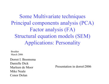
Some Multivariate techniquesPrincipal components analysis (PCA)Factor analysis (FA)Structural equation models (SEM)Applications: PersonalityBoulderMarch 2006Dorret I. BoomsmaDanielle DickMarleen de MoorMike NealeConor DolanPresentation in dorret\2006
Multivariate statistical methods; for example-Multiple regression-Fixed effects (M)ANOVA-Random effects (M)ANOVA-Factor analysis / PCA-Time series (ARMA)-Path / LISREL models
Multiple regressionx predictors (independent), e residuals, y dependent;both x and y are observedxxxxyyyeee
Factor analysis:measured and unmeasured (latent) variables. Measuredvariables can be “indicators” of unobserved traits.
Path model / SEM modelLatent traits can influence other latent traits
Measurement and causal models innon-experimental research Principal component analysis (PCA) Exploratory factor analysis (EFA) Confirmatory factor analysis (CFA) Structural equation models (SEM) Path analysisThese techniques are used to analyze multivariate data thathave been collected in non-experimental designs and ofteninvolve latent constructs that are not directly observed.These latent constructs underlie the observed variables andaccount for inter-correlations between variables.
Models in non-experimental researchAll models specify a covariance matrix Σ andmeans vector µ:Σ ΛΨΛt Θtotal covariance matrix [Σ] factor variance [ΛΨΛt ] residual variance [Θ]means vector µ can be modeled as a function ofother (measured) traits e.g. sex, age, cohort, SES
Outline Cholesky decompositionPCA (eigenvalues)Factor models (1,.4 factors)Application to personality dataScripts for Mx, [Mplus, Lisrel]
Application: personality Personality (Gray 1999): a person’s generalstyle of interacting with the world, especiallywith other people – whether one is withdrawnor outgoing, excitable or placid, conscientiousor careless, kind or stern. Is there one underlying factor? Two, three, more?
Personality: Big 3, Big 5, Big 9?Big 3Big5Big 9MPQ hievementSocial ClosenessSocial euroticismOpennessAdjustmentIntellectanceStress ReactionAbsorptionNeuroticismIndividualismLocus of Control
Data:Neuroticism, Somatic anxiety, Trait Anxiety, Beck Depression,Anxious/Depressed, Disinhibition, Boredom susceptibility, Thrillseeking, Experience seeking, Extraversion, Type-A behavior, TraitAnger, Test attitude (13 variables)Software scripts Mx (Mplus) (Lisrel)MxPersonality (also includes data)MplusLisrel Copy from dorret\2006
Cholesky decomposition for 13 personality traitsCholesky decomposition: S Q Q’where Q lower diagonal (triangular)For example, if S is 3 x 3, then Q looks like:f1lf21f310f22f3200f33I.e. # factors # variables, this approach gives a transformationof S; completely determinate.
Subjects: Birth cohorts (1909 – 1989)Four data sets were created:10001 Old male2 Young male3 Old female4 Young female800600400(N 1305)(N 1071)(N 1426)(N 1070)sexCount200femalemale00,088 ,001984 00,1980 ,001976 ,0019 2 07,01968 00,19 4 06,01960 00,1956 ,001952 ,001948 00,1944 00,1940 00,1936 00,1932 ,001928 ,0019 4 02,01920 00,190919year of birthTotal sample: 46% male, 54% femaleWhat is the structure ofpersonality?Is it the same in all datasets?
Application: Analysis of Personality in twins, spouses, sibs, parentsfrom Adult Netherlands Twin Register: longitudinal ther1071696797468Spouse of twin 1598352Total75282x3x4x2189 1471 1145844 611 3234745 3604 59425x6x867 446Total895328472739130331950868 44619529Data from multiple occasions were averaged for each subject;Around 1000 Ss were quasi-randomly selected for each sex-age groupBecause it is March 8, we use data set 3 (personShort sexcoh3.dat)
dorret\2006\Mxpersonality (docu.doc) Datafiles for Mx (and other programs; free format)personShort sexcoh1.dat old malesN 1035personShort sexcoh2.dat young malesN 1071personShort sexcoh3.dat old femalesN 1426personShort sexcoh4.dat young femalesN 1070(average yr birth 1943)(1971)(1945)(1973) Variables (53 traits): (averaged over time survey 1 – 6)trappreg trappext sex1to6 gbdjr twzyg halfsib id 2twns drieli: demographicsneu ext nso tat tas es bs dis sbl jas angs boos bdi : personalityysw ytrg ysom ydep ysoc ydnk yatt ydel yagg yoth yint yext ytot yocd: YASRcfq mem dist blu nam fob blfob scfob agfob hap sat self imp cont chck urg obs com: other Mx JobsCholesky 13vars.mx : cholesky decomposition (saturated model)Eigen 13vars.mx: eigenvalue decomposition of computed correlation matrix (alsosaturated model)Fa 1 factors.mx:1 factor modelFa 2 factors.mx :2 factor modelFa 3 factors.mx:3 factor model (constraint on loading)Fa 4 factors.mx:1 general factor, plus 3 trait factorsFa 3 factors constraint dorret.mxFa 3 factors constraint dorret.mx: alternative constraint to identify the model
title cholesky for sex/age groupsdata ng 1 Ni 53!8 demographics, 13 scales, 14 yasr, 18 extramissing -1.00!personality missing -1.00rectangular file personShort sexcoh3.datlabelstrappreg trappext sex1to6 gbdjr twzyg halfsib id 2twns drieli neu ext nso etc.Select NEU NSO ANX BDI YDEP TAS ES BS DIS EXT JAS ANGER TAT /begin matrices;A lower 13 13 free!common factorsM full 1 13 free!meansend matrices;covariance A*A'/means M /start 1.5 all etc.option nd 2end
NEU NSO ANX BDI YDEP TAS ES BS DIS EXT JAS ANGER TAT /MATRIX A: This is a LOWER TRIANGULAR matrix of order 13 by 13 -0.466.011.163.140.430.21-0.805.230.94 14.06-0.08 1.11 3.980.18 0.51 0.97 3.36-0.53 -1.21 -1.20 -1.64 7.71
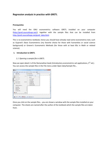
F1P1F2F3F4F5P2P3P4P5To interpret the solution, standardize the factor loadings both withrespect to the latent and the observed variables.In most models, the latent variables have unit variance;standardize the loadings by the variance of the observed variables(e.g. λ21 is divided by the SD of P2)
Group 2 in Cholesky scriptCalculate Standardized SolutionCalculationMatrices Group 1I Iden 13 13End Matrices;Begin Algebra;S (\sqrt(I.R)) ;P S*A;End Algebra;End! diagonal matrix of standard deviations! standardized estimates for factors loadings(R (A*A'). i.e. R has variances on the diagonal)
Standardized solution: standardized loadingsNEU NSO ANX BDI YDEP TAS ES BS DIS .020.020.610.26 0.760.17 -0.020.00 0.020.02 -0.010.05 -0.020.06 -0.05-0.09 -0.010.15 -0.060.19 -0.12-0.04 480.150.340.130.100.03-0.02EXT JAS ANGER TAT /0.870.24 0.940.15 0.200.07 0.210.00 0.090.01 0.05-0.05 -0.090.890.06 0.92-0.02 0.24 0.860.04 0.12 0.24 0.82-0.06 -0.14 -0.14 -0.19 0.91
NEU NSO ANX BDI YDEP TAS ES BS DIS EXT JAS ANGER TAT / Your model has104 estimated parameters :13 means13*14/2 91 factor loadings-2 times log-likelihood of data 108482.118
Eigenvalues, eigenvectors & principalcomponent analyses (PCA)1) data reduction technique2) form of factor analysis3) very useful transformation
Principal components analysis (PCA)PCA is used to reduce large set of variables into a smallernumber of uncorrelated components.Orthogonal transformation of a set of variables (x) into a setof uncorrelated variables (y) called principal components thatare linear functions of the x-variates.The first principal component accounts for as much of thevariability in the data as possible, and each succeedingcomponent accounts for as much of the remaining variabilityas possible.
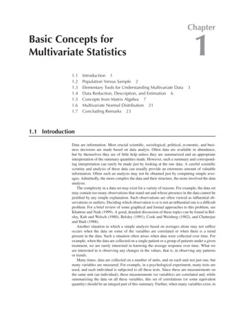
Principal component analysis of 13 personality /psychopathology inventories: 3 eigenvalues 1(Dutch adolescent and young adult twins, data 1991-1993; SPSS)43.532.521.510.50Eigenvalue
Principal components analysis (PCA)PCA gives a transformation of the correlation matrix R and is acompletely determinate model.R (q x q) P D P’, whereP q x q orthogonal matrix of eigenvectorsD diagonal matrix (containing eigenvalues)y P’ x and the variance of yj is pjThe first principal componentThe second principal componentetc.y1 p11x1 p12x2 . p1qxqy2 p21x1 p22x2 . p2qxq[p11, p12, , p1q] is the first eigenvectord11 is the first eigenvalue (variance associated with y1)
Principal components analysis (PCA)The principal components are linear combinations of thex-variables which maximize the variance of the linearcombination and which have zero covariance with theother principal components.There are exactly q such linear combinations (if R ispositive definite).Typically, the first few of them explain most of thevariance in the original data. So instead of working withX1, X2, ., Xq, you would perform PCA and then useonly Y1 and Y2, in a subsequent analysis.
PCA, Identifying constraints:transformation uniqueCharacteristics:1) var(dij) is maximal2) dij is uncorrelated with dkjare ensured by imposing the constraint:PP' P'P I (where ' stands for transpose)
Principal components analysis (PCA)The objective of PCA usually is not to account forcovariances among variables, but to summarize theinformation in the data into a smaller number of(orthogonal) variables.No distinction is made between common and uniquevariances. One advantage is that factor scores can becomputed directly and need not to be estimated.- H. Hotelling (1933): Analysis of a complex of statistical variables intoprincipal component. Journal Educational Psychology, 417-441, 498-520
PCAPrimarily data reduction technique, but often usedas form of exploratory factor analysis: Scale dependent (use only correlation matrices)! Not a “testable” model, no statistical inference Number of components based on rules of thumb(e.g. # of eigenvalues 1)
title eigen valuesdata ng 1 Ni 53missing -1.00rectangular file personShort sexcoh3.datlabelstrappreg trappext sex1to6 gbdjr twzyg halfsib id 2twns drieli neu ext nso tat tas etc.Select NEU NSO ANX BDI YDEP TAS ES BS DIS EXT JAS ANGER TAT /begin matrices;R stand 13 13 freeS diag 13 13 freeM full 1 13 freeend matrices;begin algebra;E \eval(R);V \evec(R);end algebra;covariance S*R*S'/means M /start 0.5 all etc.end!correlation matrix!standard deviations!means!eigenvalues of R!eigenvectors of R
Correlations NEU NSO ANX BDI YDEP TAS ES BS DIS EXT JAS ANGER TAT /MATRIX R: This is a STANDARDISED matrix of order 13 by 13 00.0700.045-0.0711.0000.306 1.000.172 0.1080.1910.159 ETC-0.148
Eigenvalues MATRIX E: This is a computed FULL matrixof order 13 by 1, [ \EVAL(R)] 770.7470.8240.8561.3002.0524.106What is the fit of this model?It is the same as for CholeskyBoth are saturated models
Principal components analysis (PCA): S P D P' P* P*'where S observed covariance matrixP'P I (eigenvectors)D diagonal matrix (containing eigenvalues)P* P (D1/2)Cholesky decomposition: S Q Q’where Q lower diagonal (triangular)For example, if S is 3 x 3, then Q looks like:f1lf21f310f22f3200f33If # factors # variables, Q may be rotated to P*. Both approachesgive a transformation of S. Both are completely determinate.
PCA is based on the eigenvalue decomposition.S P*D*P’If the first component approximates S:S P1*D1*P1’S Π1*Π1’, Π1 P1*D11/2It resembles the common factor modelS Σ Λ*Λ’ Θ, Λ Π1
ηy1pc1y2y3y4y1pc2 pc3 pc4y2y3y4If pc1 is large, in the sense that it accounts for much varianceηy1 y2y3y4pc1y1y2y3y4Then it resembles the common factor model (without unique variances)
Factor analysisAims at accounting for covariances among observedvariables / traits in terms of a smaller number of latentvariates or common factors.Factor Model: x Λ f e,where x observed variablesf (unobserved) factor score(s)e unique factor / errorΛ matrix of factor loadings
Factor analysis: Regression of observedvariables (x or y) on latent variables (f or η)One factor modelwith specifics
Factor analysisFactor Model: x Λ f e,With covariance matrix: Σ Λ Ψ Λ ' Θwhere Σ covariance matrixΛ matrix of factor loadingsΨ correlation matrix of factor scoresΘ (diagonal) matrix of unique variancesTo estimate factor loadings we do not need to know the individualfactor scores, as the expectation for Σ only consists of Λ, Ψ, and Θ. C. Spearman (1904): General intelligence, objectively determined and measured.American Journal of Psychology, 201-293 L.L. Thurstone (1947): Multiple Factor Analysis, University of Chicago Press
One factor model for personality? Take the cholesky script and modify it into a1 factor model (include unique variances foreach of the 13 variables) Alternatively, use the FA 1 factors.mx script NB think about starting values (look at theoutput of eigen 13 vars.mx for trait variances)
Confirmatory factor analysisAn initial model (i.e. a matrix of factor loadings) for a confirmatoryfactor analysis may be specified when for example:– its elements have been obtained from a previousanalysis in another sample.– its elements are described by a clinical model or a theoreticalprocess (such as a simplex model for repeated measures).
Mx script for 1 factor modeltitle factordata ng 1 Ni 53missing -1.00rectangular file personShort sexcoh3.datlabelstrappreg trappext sex1to6 gbdjr twzyg halfsib id 2twns drieli neu ext ETCSelect NEU NSO ANX BDI YDEP TAS ES BS DIS EXT JAS ANGER TAT /begin matrices;A full 13 1 free!common factorsB iden 1 1!variance common factorsM full 13 1 free!meansE diag 13 13 free!unique factors (SD)end matrices;specify A1 2 3 4 5 6 7 8 9 10 11 12 13covariance A*B*A' E*E'/means M /Starting valuesend
Mx output for 1 factor model1neu 21.3153nso3.7950anx7.7286bdi1.9810ydep 3.0278tas 2anger 2.1103tat-2.1191loadings Unique loadings are found on theDiagonal of E.Means are found in M matrixYour model has 39 estimated parameters-2 times log-likelihood of data 109907.19213 means13 loadings on the common factor13 unique factor loadings
Factor analysisFactor Model: x Λ f e,Covariance matrix: Σ Λ Ψ Λ ' ΘBecause the latent factors do not have a “natural” scale, the userneeds to scale them. For example:If Ψ I: Σ ΛΛ ' Θ factors are standardized to have unit variance factors are independentAnother way to scale the latent factors would be to constrain oneof the factor loadings.
In confirmatory factor analysis: a model is constructed in advance that specifies the number of (latent) factors that specifies the pattern of loadings on the factors that specifies the pattern of unique variances specific to eachobservation measurement errors may be correlated factor loadings can be constrained to be zero (or any other value) covariances among latent factors can be estimated or constrained multiple group analysis is possibleWe can TEST if these constraints are consistent with the data.
Distinctions between exploratory (SPSS/SAS)and confirmatory factor analysis (LISREL/Mx)In exploratory factor analysis: no model that specifies the number of latent factors no hypotheses about factor loadings (usually all variables loadon all factors, factor loadings cannot be constrained) no hypotheses about interfactor correlations (either nocorrelations or all factors are correlated) unique factors must be uncorrelated all observed variables must have specific variances no multiple group analysis possible under-identification of parameters
Exploratory Factor Modelf1f2f3X1X2X3X4X5X6X7e1e2e3e4e5e6e7
Confirmatory Factor Modelf1f2f3X1X2X3X4X5e1e2e3e4e5X6X7e7
Confirmatory factor analysisA maximum likelihood method for estimating the parameters in themodel has been developed by Jöreskog and Lawley (1968) andJöreskog (1969).ML provides a test of the significance of the parameter estimates andof goodness-of-fit of the model.Several computer programs (Mx, LISREL, EQS) are available. K.G. Jöreskog, D.N. Lawley (1968): New Methods in maximum likelihood factoranalysis. British Journal of Mathematical and Statistical Psychology, 85-96 K.G. Jöreskog (1969): A general approach to confirmatory maximum likelihood factoranalysis Psychometrika, 183-202 D.N. Lawley, A.E. Maxwell (1971): Factor Analysis as a Statistical Method.Butterworths, London S.A. Mulaik (1972): The Foundations of Factor analysis, McGraw-Hill Book Company,New York J Scott Long (1983): Confirmatory Factor Analysis, Sage
Structural equation modelsSometimes x Λ f e is referred to as the measurementmodel, and the part of the model that specifies relationsamong latent factors as the covariance structure model, orthe structural equation model.
Structural Modelf1f3f2X1X2X3X4X5e1e2e3e4e5X6X7e7
Path Analysis & Structural ModelsPath analysis diagrams allow us to represent linear structural models, such as regression, factoranalysis or genetic models. to derive predictions for the variances and covariances of ourvariables under that model.Path analysis is not a method for discovering causes, but a methodapplied to a causal model that has been formulated in advance. It canbe used to study the direct and indirect effects of exogenousvariables ("causes") on endogenous variables ("effects"). C.C. Li (1975): Path Analysis: A primer, Boxwood Press E.J. Pedhazur (1982): Multiple Regression Analysis Explanation and Prediction,Hold, Rinehart and Wilston
Two common factor modelη1η2Λ1,1Λ13,2y1y2y3y4y.y13e1e2e3e4e.e13
Two common factor modelyij, i 1.P tests, j 1.N casesYij λi1j η1j λi2j η2j eijΛ matrix of factor loadings:λ11 λ12λ21 λ22.λP1 λP2
IdentificationThe factor model in which all variables loadon all (2 or more) common factors is notidentified. It is not possible in the presentexample to estimate all 13x2 loadings.But how can some programs (e.g. SPSS)produce a factor loading matrix with 13x2loadings?
Identifying constraintsSpss automatically imposes the identifyingconstraint similar to:LtΘ-1L is diagonal,Where L is the matrix of factor loadings and Θ is thediagonal covariance matrix of the residuals (eij).
Other identifying constraints3 factorsλ11λ21λ31.λP10λ22λ32.λP22 here you fix the zero is not important!
Confirmatory FASpecify expected factor structure directly and fit themodel.Specification should include enough fixed parameterin Λ (i.e., zero’s) to ensure identification.Another way to guarantee identification is theconstraint that Λ Θ-1Λ’ is diagonal (this works fororthogonal factors).
2, 3, 4 factor analysis Modify an existing script (e.g. from 1 into 2 andcommon factors) ensure that the model is identified by putting at least1 zero loading in the second set of loading and atleast 2 zero’s in the third set of loadings Alternatively, do not use zero loadings but use theconstraint that Λ Θ-1Λ’ is diagonal Try a CFA with 4 factors: 1 general, 1 Neuroticism,1 Sensation seeking and 1 Extraversion factor
3 factor scriptBEGIN MATRICES;A FULL 13 3 FREEP IDEN 3 3M FULL 13 1 FREEE DIAG 13 13 FREEEND MATRICES;SPECIFY A1 0 02 14 983 15 284 16 295 17 306 18 07 19 318 20 329 21 3310 22 3411 23 3512 24 3613 25 37COVARIANCE A*P*A' E*E'/MEANS M /!COMMON FACTORS!VARIANCE COMMON FACTORS!MEANS!UNIQUE FACTORS
3 factor output:NEU NSO ANX BDI YDEP TAS ES BS DIS EXT JAS ANGER TAT / MATRIX A1 21.346123.828037.726141.990953.02296 -0.29327 0.33818 1.31999 0.889010 -4.345511 2.053912 2.080313 2.28051.8850-3.0246
Analyses 1 factor2 factor3 factor4 factor-2ll 109,097-2ll 109,082-2ll 108,728-2ll 108,782parameters 39516252 saturated-2ll 108,482104χ2 -ll(model) - -2ll(saturated;e.g. -2ll(model3) - -2ll(sat) 108,728-108,482 246; df 104-62 42
Genetic Structural Equation ModelsConfirmatory factor model: x Λ f e, wherex observed variablesf (unobserved) factor scorese unique factor / errorΛ matrix of factor loadings"Univariate" genetic factor modelP j hGj e Ej c Cj , j 1, ., n (subjects)where P measured phenotypef G: unmeasured genotypic valueC: unmeasured environment common to family membersE: unique environmentΛ h, c, e (factor loadings/path coefficients)
Genetic Structural Equation Modelsx Λf eΣ ΛΨΛ' ΘGenetic factor modelPji hGji c Cji e Eji, j 1,., n (pairs) and i 1,2 (Ss within pairs)The correlation between latent G and C factors is given in Ψ (4x4)Λ contains the loadings on G and C: h 0 c 00h0cAnd Θ is a 2x2 diagonal matrix of E factors.Covariance matrix:(MZ pairs)h*h c*c h*h c*ch*h c*c h*h c*c e*e 00 e*e
Structural equation models, summaryThe covariance matrix of a set of observed variables is a functionof a set of parameters: Σ Σ(Θ)where Σ is the population covariance matrix,Θ is a vector of model parameters andΣ is the covariance matrix as a function of ΘExample: x λf e,The observed and model covariances matrices are:Var(x)Cov(x,f) Var(f)λ2 Var(f) Var(e)λ Var(f)Var(f)KA Bollen (1990): Structural Equation with Latent Variables, John Wiley & Sons
Five steps characterize structural equation models:1. Model Specification2. Identification3. Estimation of Parameters4. Testing of Goodness of fit5. RespecificationK.A. Bollen & J. Scott Long: Testing Structural Equation Models,1993, Sage Publications
1: Model specificationMost models consist of systems of linear equations.That is, the relation between variables (latent andobserved) can be represented in or transformed tolinear structural equations. However, the covariancestructure equations can be non-linear functions of theparameters.
2: Identification: do the unknown parametersin Θ have a unique solution?Consider 2 vectors Θ1 and Θ2, each of which containsvalues for unknown parameters in Θ.If Σ(Θ1) Σ(Θ2) then the model is identified if Θ1 Θ2One necessary condition for identification is that thenumber of observed statistics is larger than or equal to thenumber of unknown parameters.(use different starting values; request CI)Identification in “twin” models depends on the multigroup design
Identification: Bivariate Phenotypes: 1 correlation and 2 variancesrGACAXAYA SYA SXhChXX1hYY1CorrelationA2hChSXX1A1hSYY1Common factorh1X1h2h3Y1Choleskydecomposition
Correlated factorsrGAXhXX1AYhYY1 Two factor loading (hx and hy)and one correlation rG Expectation:rXY hXrGhY
Common factorACA SYA SXhChChSXX1hSYY1Four factor loadings:A constraint on the factorloadings is needed tomake this modelidentified.For example: loadings onthe common factor arethe same.
Cholesky decompositionA1h1X1A2h2h3Y1 Three factor loadings If h3 0: no influencesspecific to Y If h2 0: no covariance
3: Estimation of parameters & standard errorsValues for the unknown parameters in Θ can be obtained by afitting function that minimizes the differences between the modelcovariance matrix Σ(Θ) and the observed covariance matrix S.The most general function is called Weighted Least Squares(WLS): F (s - σ) t W-1 (s - σ)where s and σ contain the non-duplicate elements of the inputmatrix S and the model matrix Σ.W is a positive definite symmetric weight matrix.The choice of W determines the fitting function.Rationale: the discrepancies between the observed and the modelstatistics are squared and weighted by a weight matrix.
Maximum likelihood estimation (MLE)Choose estimates for parameters that have the highestlikelihood given the data.A good (genetic) model should make our empirical resultslikely, if a theoretical model makes our data have a lowlikelihood of occurrence then doubt is cast on the model.Under a chosen model, the best estimates for parameters arefound (in general) by an iterative procedure that maximizes thelikelihood (minimizes a fitting function).
4: Goodness-of-fit & 5: RespecificationThe most widely used measure to assess goodness-of-fit is the chi-squaredstatistic: χ2 F (N-1), where F is the minimum of the fitting function and Nis the number of observations on which S is based.The overall χ2 tests the agreement between the observed and the predictedvariances and covariances.The degrees of freedom (df) for this test equal the number of independentstatistics minus the number of free parameters. A low χ2 with a highprobability indicates that the data are consistent with the model.Many other indices of fit have been proposed, eg Akaike's informationcriterion (AIC): χ2-2df or indices based on differences between S and Σ.Differences in goodness-of-fit between different structural equation modelsmay be assessed by likelihood-ratio tests by subtracting the chi-square of aproperly nested model from the chi-square of a more general model.
Compare models by chi square (χ²) tests:A disadvantage is that χ² is influenced by the uniquevariances of the items (Browne et al., 2002).If a trait is measured reliably, the inter-correlations ofitems are high, and unique variances are small, the χ²test may suggest a poor fit even when the residualsbetween the expected and observed data are trivial.The Standardized Root Mean-square Residual (SRMR;is a fit index that is based on the residual covariationmatrix and is not sensitive to the size of thecorrelations (Bentler, 1995).Bentler, P. M. (1995). EQS structural equations program manual. Encino, CA:Multivariate SoftwareBrowne, M. W., MacCallum, R. C., Kim, C., Andersen, B. L., & Glaser, R. (2002).When fit indices and residuals are incompatible. Psychological Methods, 7, 403-421.
Finally: factor scoresEstimates of factor loadings and unique variances can be usedto construct individual factor scores: f A’P, where A is amatrix with weights that is constant across subjects, dependingon the factor loadings and the unique variances. R.P. McDonald, E.J. Burr (1967): A comparison of four methods ofconstructing factor scores. Psychometrika, 381-401 W.E. Saris, M. dePijper, J. Mulder (1978): Optimal procedures forestimation of factor scores. Sociological Methods & Research, 85-106
Issues Distribution of the dataAveraging of data over time (alternatives)Dependency among cases (solution: correction)Final model depends on which phenotypes areanalyzed (e.g. few indicators for extraversion) Do the instruments measure the same trait in e.g.males and females (measurement invariance)?
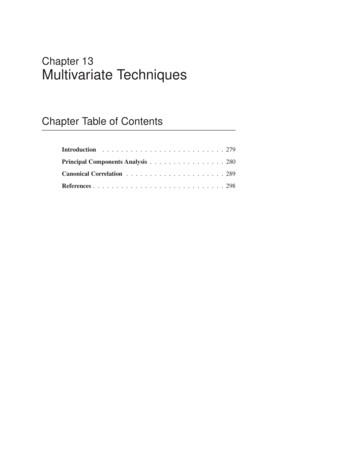
Distribution personality data(Dutch adolescent and young adult twins, data .0.0.0.0Extraversion (N 5299 0.012121110908070605040302010Neuroticism (N 5293 Ss)20.0Disinhibition (N 52813 Ss)
Beck Depression Inventory5.000Frequency4.0 003.0002 .0001.0 00Mean 1,9282Std. Dev. 2 ,72794N 10.46700,0010,0020,00bd i, 2430,00
Alternative to averaging over timeRebollo, Dolan, Boomsma
The end Scripts to run these analyses in otherprograms: Mplus and Lisrel
Exploratory factor analysis (EFA) Confirmatory factor analysis (CFA) Structural equation models (SEM) Path analysis . SPSS) 0 0.5 1 1.5 2 2.5 3 3.5 4 Eigenvalue. Principal components analysis (PCA) PCA gives a transformation of the correlation matrix R and is a completely determinate model. R (q x q) P D P', where