Transcription
This is page 383Printer: Opaque this11Vector Autoregressive Models forMultivariate Time Series11.1 IntroductionThe vector autoregression (VAR) model is one of the most successful, flexible, and easy to use models for the analysis of multivariate time series. It isa natural extension of the univariate autoregressive model to dynamic multivariate time series. The VAR model has proven to be especially useful fordescribing the dynamic behavior of economic and financial time series andfor forecasting. It often provides superior forecasts to those from univariate time series models and elaborate theory-based simultaneous equationsmodels. Forecasts from VAR models are quite flexible because they can bemade conditional on the potential future paths of specified variables in themodel.In addition to data description and forecasting, the VAR model is alsoused for structural inference and policy analysis. In structural analysis, certain assumptions about the causal structure of the data under investigation are imposed, and the resulting causal impacts of unexpected shocks orinnovations to specified variables on the variables in the model are summarized. These causal impacts are usually summarized with impulse responsefunctions and forecast error variance decompositions.This chapter focuses on the analysis of covariance stationary multivariate time series using VAR models. The following chapter describes theanalysis of nonstationary multivariate time series using VAR models thatincorporate cointegration relationships.
38411. Vector Autoregressive Models for Multivariate Time SeriesThis chapter is organized as follows. Section 11.2 describes specification,estimation and inference in VAR models and introduces the S FinMetricsfunction VAR. Section 11.3 covers forecasting from VAR model. The discussion covers traditional forecasting algorithms as well as simulation-basedforecasting algorithms that can impose certain types of conditioning information. Section 11.4 summarizes the types of structural analysis typicallyperformed using VAR models. These analyses include Granger-causalitytests, the computation of impulse response functions, and forecast errorvariance decompositions. Section 11.5 gives an extended example of VARmodeling. The chapter concludes with a brief discussion of Bayesian VARmodels.This chapter provides a relatively non-technical survey of VAR models.VAR models in economics were made popular by Sims (1980). The definitivetechnical reference for VAR models is Lütkepohl (1991), and updated surveys of VAR techniques are given in Watson (1994) and Lütkepohl (1999)and Waggoner and Zha (1999). Applications of VAR models to financialdata are given in Hamilton (1994), Campbell, Lo and MacKinlay (1997),Cuthbertson (1996), Mills (1999) and Tsay (2001).11.2 The Stationary Vector Autoregression ModelLet Yt (y1t , y2t , . . . , ynt )0 denote an (n 1) vector of time series variables.The basic p-lag vector autoregressive (VAR(p)) model has the formYt c Π1 Yt 1 Π2 Yt 2 · · · Πp Yt p εt , t 1, . . . , T(11.1)where Πi are (n n) coefficient matrices and εt is an (n 1) unobservablezero mean white noise vector process (serially uncorrelated or independent)with time invariant covariance matrix Σ. For example, a bivariate VAR(2)model equation by equation has the formµ¶µ¶ µ 1¶µ¶y1tc1π 11 π112y1t 1 (11.2)y2tc2π 121 π122y2t 1µ 2¶µ¶ µ¶π11 π212y1t 2ε1t (11.3)π221 π222y2t 2ε2tory1ty2t c1 π 111 y1t 1 π 112 y2t 1 π211 y1t 2 π212 y2t 2 ε1t c2 π 121 y1t 1 π 122 y2t 1 π221 y1t 1 π222 y2t 1 ε2twhere cov(ε1t , ε2s ) σ 12 for t s; 0 otherwise. Notice that each equationhas the same regressors — lagged values of y1t and y2t . Hence, the VAR(p)model is just a seemingly unrelated regression (SUR) model with laggedvariables and deterministic terms as common regressors.
11.2 The Stationary Vector Autoregression Model385In lag operator notation, the VAR(p) is written asΠ(L)Yt c εtwhere Π(L) In Π1 L . Πp Lp . The VAR(p) is stable if the roots ofdet (In Π1 z · · · Πp z p ) 0lie outside the complex unit circle (have modulus greater than one), or,equivalently, if the eigenvalues of the companion matrix Π1 Π2 · · · Πn In0 ···0 F . . 00. 00In0have modulus less than one. Assuming that the process has been initializedin the infinite past, then a stable VAR(p) process is stationary and ergodicwith time invariant means, variances, and autocovariances.If Yt in (11.1) is covariance stationary, then the unconditional mean isgiven byµ (In Π1 · · · Πp ) 1 cThe mean-adjusted form of the VAR(p) is thenYt µ Π1 (Yt 1 µ) Π2 (Yt 2 µ) · · · Πp (Yt p µ) εtThe basic VAR(p) model may be too restrictive to represent sufficientlythe main characteristics of the data. In particular, other deterministic termssuch as a linear time trend or seasonal dummy variables may be requiredto represent the data properly. Additionally, stochastic exogenous variablesmay be required as well. The general form of the VAR(p) model with deterministic terms and exogenous variables is given byYt Π1 Yt 1 Π2 Yt 2 · · · Πp Yt p ΦDt GXt εt(11.4)where Dt represents an (l 1) matrix of deterministic components, Xtrepresents an (m 1) matrix of exogenous variables, and Φ and G areparameter matrices.Example 64 Simulating a stationary VAR(1) model using S-PLUSA stationary VAR model may be easily simulated in S-PLUS using theS FinMetrics function simulate.VAR. The commands to simulate T 250 observations from a bivariate VAR(1) modely1ty2t 0.7 0.7y1t 1 0.2y2t 1 ε1t 1.3 0.2y1t 1 0.7y2t 1 ε2t
38611. Vector Autoregressive Models for Multivariate Time SerieswithΠ1 µ0.7 0.20.2 0.7¶, c µ 0.71.3¶, µ µ15¶, Σ µ1 0.50.5 1¶and normally distributed errors are pi1 matrix(c(0.7,0.2,0.2,0.7),2,2)mu.vec c(1,5)c.vec as.vector((diag(2)-pi1)%*%mu.vec)cov.mat matrix(c(1,0.5,0.5,1),2,2)var1.mod list(const c.vec,ar pi1,Sigma cov.mat)set.seed(301)y.var simulate.VAR(var1.mod,n 250,y0 t(as.matrix(mu.vec)))dimnames(y.var) list(NULL,c("y1","y2"))The simulated data are shown in Figure 11.1. The VAR is stationary sincethe eigenvalues of Π1 are less than one: eigen(pi1,only.values T) values:[1] 0.9 0.5 vectors:NULLNotice that the intercept values are quite different from the mean values ofy1 and y2 : c.vec[1] -0.7 1.3 colMeans(y.var)y1y20.8037 4.75111.2.1 EstimationConsider the basic VAR(p) model (11.1). Assume that the VAR(p) modelis covariance stationary, and there are no restrictions on the parameters ofthe model. In SUR notation, each equation in the VAR(p) may be writtenasyi Zπ i ei , i 1, . . . , nwhere yi is a (T 1) vector of observations on the ith equation, Z is00a (T k) matrix with tth row given by Z0t (1, Yt 1, . . . , Yt p), k np 1, π i is a (k 1) vector of parameters and ei is a (T 1) error withcovariance matrix σ 2i IT . Since the VAR(p) is in the form of a SUR model
3871011.2 The Stationary Vector Autoregression Model4-4-202y1,y268y1y2050100150200250timeFIGURE 11.1. Simulated stationary VAR(1) model.where each equation has the same explanatory variables, each equation maybe estimated separately by ordinary least squares without losing efficiencyrelative to generalized least squares. Let Π̂ [π̂ 1 , . . . , π̂ n ] denote the (k n)matrix of least squares coefficients for the n equations.Let vec(Π̂) denote the operator that stacks the columns of the (n k)matrix Π̂ into a long (nk 1) vector. That is, π̂ 1 vec(Π̂) . π̂ nUnder standard assumptions regarding the behavior of stationary and ergodic VAR models (see Hamilton (1994) or Lütkepohl (1991)) vec(Π̂) isconsistent and asymptotically normally distributed with asymptotic covariance matrix0a[var(vec(Π̂)) Σ̂ (Z Z) 1whereΣ̂ 0T1 Xε̂t ε̂0tT k t 1and ε̂t Yt Π̂ Zt is the multivariate least squares residual from (11.1) attime t.
38811. Vector Autoregressive Models for Multivariate Time Series11.2.2 Inference on CoefficientsThe ith element of vec(Π̂), π̂ i , is asymptotically normally distributed with0standard error given by the square root of ith diagonal element of Σ̂ (Z Z) 1 .Hence, asymptotically valid t-tests on individual coefficients may be constructed in the usual way. More general linear hypotheses of the formR·vec(Π) r involving coefficients across different equations of the VARmay be tested using the Wald statisticn hi o 1W ald (R·vec(Π̂) r)0 R a[(R·vec(Π̂) r) (11.5)var(vec(Π̂)) R0Under the null, (11.5) has a limiting χ2 (q) distribution where q rank(R)gives the number of linear restrictions.11.2.3 Lag Length SelectionThe lag length for the VAR(p) model may be determined using modelselection criteria. The general approach is to fit VAR(p) models with ordersp 0, ., pmax and choose the value of p which minimizes some modelselection criteria. Model selection criteria for VAR(p) models have the formIC(p) ln Σ̃(p) cT · ϕ(n, p)PTwhere Σ̃(p) T 1 t 1 ε̂t ε̂0t is the residual covariance matrix without a degrees of freedom correction from a VAR(p) model, cT is a sequence indexedby the sample size T , and ϕ(n, p) is a penalty function which penalizeslarge VAR(p) models. The three most common information criteria are theAkaike (AIC), Schwarz-Bayesian (BIC) and Hannan-Quinn (HQ):2 2pnTln T 2BIC(p) ln Σ̃(p) pnT2 ln ln T 2HQ(p) ln Σ̃(p) pnTThe AIC criterion asymptotically overestimates the order with positiveprobability, whereas the BIC and HQ criteria estimate the order consistently under fairly general conditions if the true order p is less than orequal to pmax . For more information on the use of model selection criteriain VAR models see Lütkepohl (1991) chapter four.AIC(p) ln Σ̃(p) 11.2.4 Estimating VAR Models Using the S FinMetricsFunction VARThe S FinMetrics function VAR is designed to fit and analyze VAR modelsas described in the previous section. VAR produces an object of class “VAR”
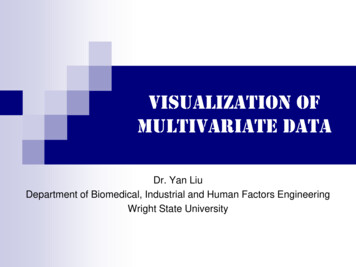
11.2 The Stationary Vector Autoregression Model389for which there are print, summary, plot and predict methods as wellas extractor functions coefficients, residuals, fitted and vcov. Thecalling syntax of VAR is a bit complicated because it is designed to handlemultivariate data in matrices, data frames as well as “timeSeries” objects.The use of VAR is illustrated with the following example.Example 65 Bivariate VAR model for exchange ratesThis example considers a bivariate VAR model for Yt ( st , f pt )0 ,where st is the logarithm of the monthly spot exchange rate between the USSand Canada, f pt ft st iU iCAis the forward premium or interestttrate differential, and ft is the natural logarithm of the 30-day forwardexchange rate. The data over the 20 year period March 1976 through June1996 is in the S FinMetrics “timeSeries” lexrates.dat. The data forthe VAR model are computed as dspot diff(lexrates.dat[,"USCNS"])fp ts seriesMerge(dspot,fp)colIds(uscn.ts) c("dspot","fp")uscn.ts@title "US/CN Exchange Rate Data"par(mfrow c(2,1))plot(uscn.ts[,"dspot"],main "1st difference of US/CA spotexchange rate")plot(uscn.ts[,"fp"],main "US/CN interest ratedifferential")Figure 11.2 illustrates the monthly return st and the forward premiumf pt over the period March 1976 through June 1996. Both series appear to beI(0) (which can be confirmed using the S FinMetrics functions unitrootor stationaryTest) with st much more volatile than f pt . f pt also appears to be heteroskedastic.Specifying and Estimating the VAR(p) ModelTo estimate a VAR(1) model for Yt use var1.fit VAR(cbind(dspot,fp) ar(1),data uscn.ts)Note that the VAR model is specified using an S-PLUS formula, with themultivariate response on the left hand side of the operator and the builtin AR term specifying the lag length of the model on the right hand side.The optional data argument accepts a data frame or “timeSeries” object with variable names matching those used in specifying the formula.If the data are in a “timeSeries” object or in an unattached data frame(“timeSeries” objects cannot be attached) then the data argument mustbe used. If the data are in a matrix then the data argument may be omitted. For example,
39011. Vector Autoregressive Models for Multivariate Time Series-0.06-0.020.021st difference of US/CN spot exchange rate1976 1977 1978 1979 1980 1981 1982 1983 1984 1985 1986 1987 1988 1989 1990 1991 1992 1993 1994 1995 1996-0.005-0.0010.003US/CN interest rate differential1976 1977 1978 1979 1980 1981 1982 1983 1984 1985 1986 1987 1988 1989 1990 1991 1992 1993 1994 1995 1996FIGURE 11.2. US/CN forward premium and spot rate. uscn.mat as.matrix(seriesData(uscn.ts)) var2.fit VAR(uscn.mat ar(1))If the data are in a “timeSeries” object then the start and end optionsmay be used to specify the estimation sample. For example, to estimate theVAR(1) over the sub-period January 1980 through January 1990 var3.fit VAR(cbind(dspot,fp) ar(1), data uscn.ts, start "Jan 1980", end "Jan 1990", in.format "%m %Y")may be used. The use of in.format \%m %Y" sets the format for the datestrings specified in the start and end options to match the input formatof the dates in the positions slot of uscn.ts.The VAR model may be estimated with the lag length p determined usinga specified information criterion. For example, to estimate the VAR for theexchange rate data with p set by minimizing the BIC with a maximum lagpmax 4 use var4.fit VAR(uscn.ts,max.ar 4, criterion "BIC") var4.fit infoar(1) ar(2) ar(3) ar(4)BIC -4028 -4013 -3994 -3973When a formula is not specified and only a data frame, “timeSeries” ormatrix is supplied that contains the variables for the VAR model, VAR fits
11.2 The Stationary Vector Autoregression Model391all VAR(p) models with lag lengths p less than or equal to the value givento max.ar, and the lag length is determined as the one which minimizesthe information criterion specified by the criterion option. The defaultcriterion is
godic VAR models (see Hamilton (1994) or L utkepohl (1991)) vec(Πˆ)is consistent and asymptotically normally distributed with asymptotic covari-ance matrix 0 Z) 1 where Σˆ 1 T k XT t 1 ˆε t ˆε 0 and ˆεt Yt 0 Ztis the multivariate least squares residual from (11.1) at time t. 388 11. Vector Autoregressive Models for Multivariate Time Series 11.2.2 Inference on Coefficients The .