Transcription
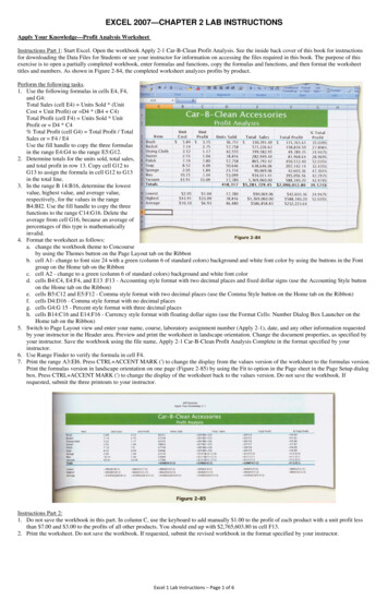
EXCEL 2007—CHAPTER 2 LAB INSTRUCTIONSApply Your Knowledge—Profit Analysis WorksheetInstructions Part 1: Start Excel. Open the workbook Apply 2-1 Car-B-Clean Profit Analysis. See the inside back cover of this book for instructionsfor downloading the Data Files for Students or see your instructor for information on accessing the files required in this book. The purpose of thisexercise is to open a partially completed workbook, enter formulas and functions, copy the formulas and functions, and then format the worksheettitles and numbers. As shown in Figure 2-84, the completed worksheet analyzes profits by product.Perform the following tasks.1. Use the following formulas in cells E4, F4,and G4:Total Sales (cell E4) Units Sold * (UnitCost Unit Profit) or D4 * (B4 C4)Total Profit (cell F4) Units Sold * UnitProfit or D4 * C4% Total Profit (cell G4) Total Profit / TotalSales or F4 / E4Use the fill handle to copy the three formulasin the range E4:G4 to the range E5:G12.2. Determine totals for the units sold, total sales,and total profit in row 13. Copy cell G12 toG13 to assign the formula in cell G12 to G13in the total line.3. In the range B 14:B16, determine the lowestvalue, highest value, and average value,respectively, for the values in the rangeB4:BI2. Use the fill handle to copy the threefunctions to the range C14:G16. Delete theaverage from cell G16, because an average ofpercentages of this type is mathematicallyinvalid.4. Format the worksheet as follows:a. change the workbook theme to Concourseby using the Themes button on the Page Layout tab on the Ribbonb. cell A1- change to font size 24 with a green (column 6 of standard colors) background and white font color by using the buttons in the Fontgroup on the Home tab on the Ribbonc. cell A2 - change to a green (column 6 of standard colors) background and white font colord. cells B4:C4, E4:F4, and E13 :F13 - Accounting style format with two decimal places and fixed dollar signs (use the Accounting Style buttonon the Home tab on the Ribbon)e. cells B5:C12 and E5:F12 - Comma style format with two decimal places (use the Comma Style button on the Home tab on the Ribbon)f. cells D4:D16 - Comma style format with no decimal placesg. cells G4:G 15 - Percent style format with three decimal placesh. cells B14:C16 and E14:F16 - Currency style format with floating dollar signs (use the Format Cells: Number Dialog Box Launcher on theHome tab on the Ribbon)5. Switch to Page Layout view and enter your name, course, laboratory assignment number (Apply 2-1), date, and any other information requestedby your instructor in the Header area. Preview and print the worksheet in landscape orientation. Change the document properties, as specified byyour instructor. Save the workbook using the file name, Apply 2-1 Car-B-Clean Profit Analysis Complete in the format specified by yourinstructor.6. Use Range Finder to verify the formula in cell F4.7. Print the range A3:EI6. Press CTRL ACCENT MARK (') to change the display from the values version of the worksheet to the formulas version.Print the formulas version in landscape orientation on one page (Figure 2-85) by using the Fit to option in the Page sheet in the Page Setup dialogbox. Press CTRL ACCENT MARK (') to change the display of the worksheet back to the values version. Do not save the workbook. Ifrequested, submit the three printouts to your instructor.Instructions Part 2:1. Do not save the workbook in this part. In column C, use the keyboard to add manually 1.00 to the profit of each product with a unit profit lessthan 7.00 and 3.00 to the profits of all other products. You should end up with 2,765,603.80 in cell F13.2. Print the worksheet. Do not save the workbook. If requested, submit the revised workbook in the format specified by your instructor.Excel 1 Lab Instructions – Page 1 of 6
Extend Your Knowledge—Applying Conditional Formatting to CellsInstructions: Start Excel. Open the workbook Extend 2-1 Biology 201 Midterm Scores. See the inside back cover of this book for instructions fordownloading the Data Files for Students, or see your instructor for information on accessing the files required in this book. Perform the followingtasks to apply new conditional formatting to the worksheet.1. Select the range C4:C18. Click the Conditional Formatting button on theHome tab on the Ribbon and then select New Rule in the ConditionalFormatting gallery. Select 'Format only top or bottom ranked values' in theSelect a Rule Type area (Figure 2-86). Enter a value between 20 and 35 ofyour choosing in the text box in the Edit the Rule Description area andclick the '% of the selected range' check box to select it. Click the Formatbutton and choose a format to assign to this conditional format. Click theOK button in each dialog box to close the dialog boxes and view theworksheet.2. With range C4:C18 selected, apply a conditional format to the range thathighlights scores that are below average.3. With range D4:D18 selected, apply a conditional format to the range thathighlights any grade that is a D or an F.4. With range B4:B18 selected, apply a conditional format to the range thatuses a red color to highlight any duplicate student names.5. Change the document properties, as specified by your instructor. Changethe worksheet header with your name, course number, and otherinformation requested by your instructor. Save the workbook using the filename, Extend 2-1 Biology 201 Midterm Scores Complete, and submit therevised workbook as Specified by your instructor.Make It Right—Correcting Functions and Formulas in a WorksheetInstructions: Start Excel. Open the workbook Make It Right 2-1 El Centro Diner Payroll Report. See the inside back cover of this book forinstructions for downloading the Data Files for Students, or see your instructor for information on accessing the files required for this book. Correctthe following formatting, function, and formula problems (Figure 2-87) in the worksheet.1. Adjust the width of column B to 11.25 pixels so that the word in the column header does not wrap.2. Spell check the worksheet and correct any spelling mistakes that are found, but ignore any spelling mistakes found with the worksheet title andthe employee names.3. The averages in several columns do not include the employee in row 13. Adjust the functions in these cells so that all employees are included inthe calculation.4. The net pay calculation should be:Net Pay Gross Pay - (Federal Taxes State Taxes)Adjust the formulas in the range H4:H13 so that the correct formula is used.5. The value for the highest value in column C was entered as a number rather than as a function. Replace the value with the appropriate function.6. The currency values in row 4 should be formatted with the Accounting Number Format button on the Home tab on the Ribbon. They arecurrently formatted with the Currency format.7. Delete the function in the cell containing the average of % Taxes because it is mathematically invalid.8. Change the document properties, as specified by your instructor. Change the worksheet header with your name, course number, and otherinformation requested by your instructor. Save the workbook using the file name, Make It Right 2-1 El Centro Diner Payroll Report Corrected.Submit the revised workbook as specified by your instructor.Excel 1 Lab Instructions – Page 2 of 6
Lab 1: Sales Analysis WorksheetProblem: You have been asked to build a sales analysis worksheet for Facade Importers that determines the sales quota and percentage of quota metfor the sales representatives in Table 2-8. The desired worksheet is shown in Figure 2-88.Instructions Part 1: Perform the following tasks to build the worksheet shown in Figure 2-88.1. Apply the Aspect theme to theworksheet by using the Themesbutton on the Page Layout tab onthe Ribbon.2. Increase the width of column Ato 19.00 points and the width ofcolumns B through F to 13.50points.3. Enter the worksheet title FacadeImporters in cell Al and theworksheet subtitle SalesAnalysis in cell A2. Enter thecolumn titles in row 3 as shownin Figure 2-88. In row 3, useALT ENTER to start a new linein a cell.4. Enter the sales data described inTable 2-8 in columns A, B, C,and E in rows 4 through 9. Enterthe row titles in the rangeA10:A14 as shown in Figure 288 on the previous page.5. Obtain the net sales in column Dby subtracting the sales returnsin column C from the salesamount in column B. Enter the formula in cell D4 and copy it to the range DS:D9.6. Obtain the above quota amounts in column F by subtracting the sales quota in column E from the net sales in column D. Enter the formula in cellF4 and copy it to the range FS:F9.7. Obtain the totals in row 10 by adding the column values for each salesperson. In the range B11:B13, use the AVERAGE, MAX, and MINfunctions to determine the average, highest value, and lowest value in the range B4:B9. Copy the range B11:B13 to the range C11:F13.8. Determine the percent of quota sold in cell B 14 by dividing the total net sales amount in cell D 1 0 by the total sales quota amount in cell E10.Center this value in the cell.9. If necessary, click the Home tab on the Ribbon. One at a time, merge and center the worksheet title and subtitle across columns A through F.Select cells Al and A2 and change the background color to red (column 2 in the Standard Colors area on the Fill Color palette). Apply the Titlecell ' style to cells Al and B1 by clicking the Cell Styles button on the Home tab on the Ribbon and clicking the Title cell style in the Titles andHeadings area in the Cell Styles gallery. Change the worksheet title in cell Al to 2 8-point white (column 1, row 1 on the Font Color gallery).Change the worksheet subtitle to the same color. Assign a thick box border from the Borders gallery to the range A1:A2.10. Center the titles in row 3, columns A through F. Apply the Heading 3 cell style to the range A3:F3. Use the Italic button on the Home tab on theRibbon to italicize the column titles in row 3 and the row titles in the range A10:A14.11. Apply the Total cell style to the range A10:F10. Assign a thick box to cell B14. Change the background and font colors for cell B14 to the samecolors applied to the worksheet title in Step 9.12. Change the row heights of row 3 to 33.00 points and rows 11 and 14 to 30.00 points.13. Select cell B14 and then click the Percent Style button on the Home tab on the Ribbon. Click the Increase Decimal button on the Ribbon twice todisplay the percent in cell B14 to hundredths.14. Use the CTRL key to select the ranges B4:F4 and B10:F13. That is, select the range B4:F4 and then while holding down the CTRL key, select therange B10:F13. Use the Format Cells: Number Dialog Box Launcher button on the Home tab on the Ribbon to display the Format Cells dialogbox to assign the selected ranges a Floating Dollar Sign style format with two decimal places and parentheses to represent negative numbers.Select the range B5:F9 and click the Comma Style button on the Home tab on the Ribbon.15. Rename the sheet tab as Sales Analysis. Change the document properties, as specified by your instructor. Change the worksheet header with yourname, course number, and other information requested by your instructor.16. Save the workbook using the file name Lab 2-1 Part 1 Facade Importers Sales Analysis. Print the entire worksheet in landscape orientation. Printonly the range A3:B10.17. Display the formulas version by pressing CTRL ACCENT MARK n. Print the formulas version using the Fit to option button in the Scaling areaon the Page tab in the Page Setup dialog box. After printing the worksheet, reset the Scaling option by selecting the Adjust to option button on thePage tab in the Page Setup dialog box and changing the percent value to 100%. Change the display from the formulas version to the valuesversion by pressing CTRL ACCENT MARK ( ). Do not save the workbook.18. Submit the assignment as specified by your instructor.Instructions Part 2: Open the workbook created in Part 1 and save the workbook as Lab 2-1 Part 2 Facade Importers Sales Analysis. Manuallydecrement each of the six values in the sales amount column by 10,000.00 until the percent of quota sold in cell B14 is below, yet as close aspossible to, 100%. All six values in column B must be incremented the same number of times. The percent of quota sold in B14 should equal99.85%. Update the worksheet header and save the workbook. Print the worksheet. Submit the assignment as specified by your instructor.Excel 1 Lab Instructions – Page 3 of 6
Instructions Part 3: Open the workbook created in Part 2 and then save the workbook as Lab 2-1 Part 3 Facade Importers Sales Analysis. With thepercent of quota sold in cell B14 equal to 99.85% from Part 2, manually decrement each of the six values in the sales return column by 1,000.00until the percent of quota sold in cell B 14 is above, yet as close as possible to, 100%. Decrement all six values in column C the same number oftimes. Your worksheet is correct when the percent of quota sold in cell B14 is equal to 100.12%. Update the worksheet header and save theworkbook. Print the worksheet. Submit the assignment as specified by your instructor.Lab 2: Balance Due WorksheetProblem: You are a spreadsheet intern for Jackson's Bright Ideas, a popular Denver-based light fixture store with outlets in major cities across thewestern United States. You have been asked to use Excel to generate a report (Figure 2-89) that summarizes the monthly balance due. A graphicbreakdown of the data also is desired. The customer data in Table 2-9 is available for test purposes.Instructions Part 1: Create a worksheet similar to the one shown in Figure 2-89. Include the five columns of customer data in Table 2-9 in the report,plus two additional columns to compute a service charge and a new balance for each customer. Assume no negative unpaid monthly balances.Perform the following tasks:1. Enter and format the worksheet title Jackson's Bright Ideas and worksheet subtitle Monthly Balance Due Report in cells Al and A2. Change thetheme of the worksheet to the Technic theme. Apply the Title cell style to cells Al and A2. Change the font size in cell A1 to 28 points. One at atime, merge and center the worksheet title and subtitle across columns A through G. Change the background color of cells A1 and A2 to yellow(column 4 in the Standard t Colors area in the Font Color palette). Draw a thick box border around the range A1:A2.2. Change the width of column Ato 20.00 characters. Change thewidths of columns B through Gto 12.00. Change the heights ofrow 3 to 36.00 and row 12 to30.00 points.3. Enter the column titles in row 3and row titles in the rangeA11:A14 as shown in Figure 289. Center the column titles inthe range A3:G3. Apply theHeading 3 cell style to therange A3:G3. Bold the titles inthe range A11:A14. Apply theTotal cell style to the rangeA11:G11. Change the font sizeof the cells in the rangeA3:G14 to 12 points.4. Enter the data in Table 2-9 inthe range A4:E10.5. Use the following formulas todetermine the service charge incolumn F and the new balance in column G for the first customer. Copy the two formulas down through the remaining customers.a. Service Charge (cell F4) 2.75% * (Beginning Balance - Payments - Credits) or 0.0275 * (B4 - D4 - C4)b. New Balance (G4) Beginning Balance Purchases - Credits - Payments Service Charge or B4 E4 - C4 - D4 F46. Determine the totals in row 11.7. Determine the maximum, minimum, and average values in cells B 12:B14 for the range B4:B10 and then copy the range B12:B14 to C12:G14.8. Use the Format Cells command on the shortcut menu to format the numbers as follows: (a) assign the Currency style with a floating dollar sign tothe cells containing numeric data in the ranges B4:G4 and B11:G14; and (b) assign the Comma style (currency with no dollar sign) to the rangeB5:G10.9. Use conditional formatting to change the formatting to white font on a red background in any cell in the range C4:C10 that contains a valuegreater than 50.10. Change the worksheet name from Sheet 1 to Balance Due. Change the document properties, as specified by your instructor. Change theworksheet header with your name, course number, and other information requested by your instructor.11. Spell check the worksheet. Preview and then print the worksheet in landscape orientation. Save the workbook using the file name, Lab 2-2 Part 1Jackson's Bright Ideas Monthly Balance Due Report.12. Print the range A3:D14. Print the formulas version on one page. Close the workbook without saving the changes. Submit the assignment asspecified by your instructor.Excel 1 Lab Instructions – Page 4 of 6
Instructions Part 2: This part requires that a 3-D Bar chart with a cylindrical shape be inserted on a new worksheet in the workbook. If necessary, useExcel Help to obtain information on inserting a chart on a separate sheet in the workbook.1. With the Lab 2-2 Part 1 Jackson's Bright Ideas Monthly Balance Due Report workbook open, save the workbook using the file name, Lab 2-2Part 2 Jackson's Bright Ideas Monthly Balance Due Report. Draw the 3-D Bar chart with cylindrical shape showing each customer's total newbalance as shown in Figure 2-90.2. Use the CTRL key and mouse to select the nonadjacent chart ranges A4:A10 and G4:G10. That is, select the range A4:A10 and then whileholding down the CTRL key, select the range G4:G10. The Customer names in the range A4:A10 will identify the cylindrical bars, while the dataseries in the range G4:G10 will determine the length of the bars.3. Click the Insert tab on the Ribbon. Click the Bar button in the Charts group on the Ribbon and then select Clustered Horizontal Cylinder in theCylinder area. When the chartis displayed on the worksheet,click the Move Chart button onthe Ribbon. When the MoveChart dialog box appears, clickNew sheet and then type BarChart for the sheet name. Clickthe OK button.4. When the chart is displayed onthe new worksheet, click thechart area, which is a blankarea near the edge of the chart,and then click the Formatcontextual tab. Click the ShapeFill button on the Ribbon andthen select Gold, Accent 2,Lighter 80% in the gallery(column 6, row 2). Click theLayout contextual tab. Clickthe Chart Title button on theRibbon and then select AboveChart in the Chart Title gallery.If necessary, use the scroll baron the right side of theworksheet to scroll to the top ofthe chart. Click the edge of thechart title to select it and then type Balance Due as the chart title.5. Drag the Balance Due tab at the bottom of the worksheet to the left of the Bar Chart tab to reorder the sheets in the workbook. Preview and printthe chart.6. Click the Balance Due sheet tab. Change the following purchases: customer John McCartan to 406.58, and customer Pam Paoli to 74.99. Thecompany also decided to change the service charge from 2.75% to 3.25% for all customers. After copying the adjusted formula in cell F4 to therange F5:F10, click the Auto Fill Options button and then click Fill without Formatting to maintain the original formatting in the range F5:F10.The total new balance in cell G11 should equal 2,919.01.7. Select both sheets by holding down the SHIFT key and then clicking the Bar Chart tab. Preview and print the selected sheets. Submit theassignment as requested by your instructor. Save the workbook.8. Submit the assignment as specified by your instructor.Instructions Part 3: With your instructor's permission, e-mail the workbook created in this exercise with the changes indicated in Part 2 as anattachment to your instructor. Close the workbook without saving the changes.Excel 1 Lab Instructions – Page 5 of 6
Lab 3: Equity Web QueriesProblem: A friend of your family, Benson Yackley, has learned that Excel can connect to the Web, download real-time stock data into a worksheet,and then refresh the data as often as needed. Because you have had courses in Excel and the Internet, he has hired you as a consultant to develop astock analysis workbook. His portfolio is shown in Table 2-10.Instructions Part 1: Start Excel. If necessary, connect to the Internet. Perform a Web query to obtain multiple stock quotes (Figure 2-91), using thestock symbols in the second column of Table 2-10. Place the results of the Web query in a new worksheet. Rename the worksheet Real-Time StockQuotes. Change the document properties, as specified by your instructor. Save the workbook using the file name, Lab 2-3 Part 1 Benson YackleyEquities Online. Preview and then print the worksheet in landscape orientation using the Fit to option.Click the following links and print the Web page that appears in the browser window: Click here to visit MSN Money; Dell Inc.; Chart (to the rightof MetLife, Inc.); and News (to the right of PepsiCo, Inc.). Submit the assignment as specified by your instructorInstructions Part 2: While connected to the Internet and with the Lab 2-3 Benson Yackley Equities Online workbook open, create a worksheet listingthe major indices and their current values on Sheet2 of the workbook (Figure 2-92). After clicking the Sheet2 tab, create the worksheet by doubleclicking MSN MoneyCentral Investor Major Indices in the Existing Connections dialog box. The dialog box is displayed when you click the ExistingConnections button on the Data tab on the Ribbon. Rename the worksheet Major Indices. Preview and then print the Major Indices worksheet inlandscape orientation using the Fit to option. Save the workbook using the same file name as in Part 1. Submit the assignment as specified by yourinstructor.Excel 1 Lab Instructions – Page 6 of 6
Excel 1 Lab Instructions – Page 3 of 6 Lab 1: Sales Analysis Worksheet Problem: You have been asked to build a sales analysis worksheet for Facade Importers that determines the sales quota and percentage of quota met for the sales representatives in
