WIXLIB

Multivariate Data AnalysisSusan Holmes http://www-stat.stanford.edu/ susan/Bio-X and StatisticsIMA Workshop, October, 2013ABabcdfghiejkl. . . . . . . . . . . . . .

you do not really understand something unless you canexplain it to your grandmother -- Albert Einstein. . . . . . . . . . . . . .

you do not really understand something unless you canexplain it to your grandmother -- Albert EinsteinI am your grandmother . . . . . . . . . . . . . .

What are multivariate data ?Simplest format: matrices:If we have measured 10,000 genes on hundreds of patientsand all the genes are independent, we can't do better thananalyze each gene's behavior by using histograms or boxplots, looking at the means, medians, variances and other onedimensional statistics'. However if some of the genes areacting together, either that they are positively correlated orthat they inhibit each other, we will miss a lot of importantinformation by slicing the data up into those column vectorsand studying them separately. Thus important connectionsbetween genes are only available to us if we consider thedata as a whole. We start by giving a few examples of datathat we encounter. . . . . . . . . . . . . .

Athletes, performances in the decathlon.100 long poid haut 400 110 disq perc jave 151 11.25 7.43 15.48 2.27 48.90 15.13 49.28 4.7 61.322 10.87 7.45 14.97 1.97 47.71 14.46 44.36 5.1 61.763 11.18 7.44 14.20 1.97 48.29 14.81 43.66 5.2 64.164 10.62 7.38 15.02 2.03 49.06 14.72 44.80 4.9 64.045 11.02 7.43 12.92 1.97 47.44 14.40 41.20 5.2 57.46 Clinical measurements (diabetes data).13579 relwt glufast glutest steady insulin 4330.9110035022111930.9997379142983OTU read counts:EKCM1.489478EKCM7.489464EKBM2.489466469478 208196 378462 265971 5708120020000202. . .000 . . .12. . . .0. . . . . .

PTCM3.489508EKCF2.489571 00001440000RNA-seq, transcriptomic:FBgn0000017 FBgn0000018 FBgn0000022 308051 Mass spec:Samples Features.mz129.9816KOGCHUM1 60515WTGCHUM1 252579WTGCHUM2 18785972.08144 151.6255 142.0349 169.04131814950196526255005154697412487800487751. . .45626.5631846425. . . . .454226. . . . . . 1

DependenciesIf the data were all independent columns, then the data wouldhave no multivariate structure and we could just do univariatestatistics on each variable (column) in turn.Multivariate statistics means we are interested in how the columnscovary.We can compute covariances to evaluate the dependencies.If the data were multivariate normal with p variables, all theinformation would be contained in the p p covariance matrix Σand the mean µ. . . . . . . . . . . . . .

Parametric Multivariate Normal. . . . . . . . . . . . . .

Modern Statistics: Non parametric, multivariate Exploratory Analyses: Hypotheses generating. Projection Methods (new coordinates)Principal Component AnalysisPrincipal Coordinate Analysis-Multidimensional Scaling(PCO,MDS)Correspondence AnalysisDiscriminant AnalysisTree based methodsPhylogenetic TreesClustering TreesDecision TreesConfirmatory Analyses: Hypothesis verification. Permutation tests (Monte Carlo). Bootstrap (Monte Carlo). Bayesian nonparametrics (Monte Carlo). . . . . . . . . . . . . .

Modern Methods: Robust MethodsVarianceVariability of one continuous variable the variance.NOT ROBUST, low breakdown.Solution: Take ranks, clumps, logs, or trimming the data. . . . . . . . . . . . . .

Part IEDA: Exploratory Data AnalysisData CheckingHypothesis Generating. . . . . . . . . . . . . .

Discovery by Visualizationd 0.02 1 3 2 . . . . . . . . . . . . . .

Basic Visualization Tools Boxplots, barplots. Scatterplots of projected data. Scatterplots with binning variable Hierarchical Clustering, heatmaps, Phylogenies. Combination of Phylogenetic Trees and data. . . . . . . . . . . . . .

Iterative Structuration (Tukey, 1977). . . . . . . . . . . . . .

One table methods: PCA, MDS, PCoA, CA, ablesobservationsendAll based on the principle of finding the largest axis ofinertia/variability.New Variables/coordinates from old or distancesBest Projection Directions?. . . . . . . . . . . . . .

. . . . . . . . . . . . . .

. . . . . . . . . . . . . .

PCA oicevariablesobservationsendAll based on the principle of finding the largest axis ofinertia/variability.New Variables/coordinates from old or distancesBest Projection Directions because they explain the most variance. . . . . . . . . . . . . .

Our first task is often to rescale the data so that all thevariables, or columns of the matrix have the same standarddeviation, this will put all the variables on the same footing.We also make sure that the means of all columns are zero,this is called centering. After that we will try to simplify thedata by doing what we call rank reduction, we'll explain thisconcept from several different perspectives. A favorite toolfor simplifying the data is called Principal Component Analysis(abbreviated PCA). . . . . . . . . . . . . .

What is PCA?PCA is an unsupervised learning technique' because it treats allvariables as having the same status, there is no particular responsevariable that we are trying to predict using the other variables asexplanatory predictors as in supervised methods. PCA is primarily avisualization technique which produces maps that show therelations between the variables in a useful way. . . . . . . . . . . . . .

Useful Facts to Remember Each PC is defined to maximize the variance it explains. The new variables are made to be orthogonal, if the dataare multivariate normal they will be independent. Always check the screeplot before deciding how manycomponents to retain (how much signal you have). . . . . . . . . . . . . .

A Geometrical Approachi. The data are p variables measured on n observations.ii. X with n rows (the observations) and p columns (thevariables).iii. Dn is an n n matrix of weights on the observations'',which is most often diagonal.iv Symmetric definite positive matrix Q,often 1σ12 0 Q 0.01σ220.001σ32.0000 . . 1σp2. . . . . . . . . . . . . .

Euclidean SpacesThese three matrices form the essential triplet" (X, Q, D) defininga multivariate data analysis.Q and D define geometries or inner products in Rp and Rn ,respectively, throughxt Qy x, y Qx , y Rpxt Dy x, y Dx , y Rn . . . . . . . . . . . . . .

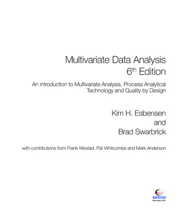
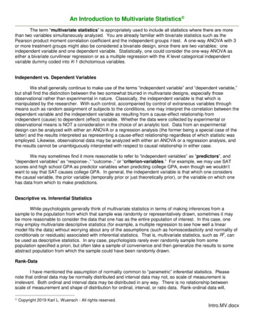
An Algebraic Approach Q can be seen as a linear function from Rp toRp L(Rp ), the space of scalar linear functions on Rp .D can be seen as a linear function from Rn toRn L(Rn ).Rp RnXx x Q DyyV WRp XtRn . . . . . . . . . . . . . .

An Algebraic ApproachRp RnXx x Q DyyV WRp XtRn Duality diagrami. Eigendecomposition of Xt DXQ VQii. Eigendecomposition of XQXt D WDiii. Transition Formulae. . . . . . . . . . . . . .

Notes(1) Suppose we have data and inner products defined by Q and D :(x, y) Rp Rp 7 xt Qy x, y Q R(x, y) Rn Rn 7 xt Dy x, y D R. x 2Q x, x Q p j 1qj (x.j )2 x 2D x, x D p pi (xi. )2j 1(2) We say an operator O is B-symmetric if x, Oy B Ox, y B ,or equivalently BO Ot B.The duality diagram is equivalent to (X, Q, D) such that X is n p .Escoufier (1977) defined as XQXt D WD and Xt DXQ VQ as thecharacteristic operators of the diagram. . . . . . . . . . . . . .

(3) V Xt DX will be the variance-covariance matrix, if X iscentered with regards to D (X′ D1n 0). . . . . . . . . . . . . .

Transposable DataThere is an important symmetry between the rows and columns ofX in the diagram, and one can imagine situations where the role ofobservation or variable is not uniquely defined. For instance inmicroarray studies the genes can be considered either as variablesor observations. This makes sense in many contemporary situationswhich evade the more classical notion of n observations seen as arandom sample of a population. It is certainly not the case thatthe 9,000 species are a random sample of bacteria since theseprobes try to be an exhaustive set. . . . . . . . . . . . . .

Two Dual Geometries. . . . . . . . . . . . . .

Properties of the DiagramRank of the diagram: X, Xt , VQ and WD all have the same rank.For Q and D symmetric matrices, VQ and WD are diagonalisableand have the same eigenvalues.λ1 λ2 λ3 . . . λr 0 · · · 0.Eigendecomposition of the diagram: VQ is Q symmetric, thus wecan find Z such thatVQZ ZΛ, Zt QZ Ip , where Λ diag(λ1 , λ2 , . . . , λp ).(1). . . . . . . . . . . . . .

Practical ComputationsCholesky decompositions of Q and D, (symmetric and positivedefinite) Ht H Q and Kt K D.Use the singular value decomposition of KXH:KXH USTt ,with Tt T Ip , Ut U In , S diagonal.Then Z (H 1 )t T satisfiesVQZ ZΛ, Zt QZ Ipwith Λ S2 .The renormalized columns of Z, A SZ are called the principalaxes and satisfy:At QA Λ. . . . . . . . . . . . . .

Practical ComputationsSimilarly, we can define L K 1 U that satisfiesWDL LΛ, Lt DL In , where Λ diag(λ1 , λ2 , . . . , λr , 0, . . . , 0). (2)C LS is usually called the matrix of principal components. It isnormed so thatCt DC Λ. . . . . . . . . . . . . .

Transition Formulæ:Of the four matrices Z, A, L and C we only have to compute one, allothers are obtained by the transition formulæ provided by theduality property of the diagram:XQZ LS CXt DL ZS A. . . . . . . . . . . . . .

General Features1. Inertia : Trace(VQ) Trace(WD)(inertia in the sense of Huyghens inertia formula for instance).Huygens, C. (1657),n pi d2 (xi , a)i 1Inertia with regards to a point a of a cloud of pi -weighted points.PCA with Q Ip , D 1n In , and the variables are centered, theinertia is the sum of the variances of all the variables.If the variables are standardized (Q is the diagonal matrix ofinverse variances), then the inertia is the number of variables p.For correspondence analysis the inertia is the Chi-squared statistic. . . . . . . . . . . . . .

Ordination MethodsMany discrete measurements Gradients.Data from 2005 U.S. House of Representatives roll call votes. Wefurther restricted our analysis to the 401 Representatives thatvoted on at least 90% of the roll calls (220 Republicans, 180Democrats and 1 Independent) leading to a 401 669 matrix V ofvoting data. . . . . . . . . . . . . .

The 1V311-1-1-1111-11V4-1-1111-1-1-11-1V5 V6 V7 V8 V9 V100 1 1 1 110 1 1 1 11-1 1 1 -1 -1 -1-1 1 1 -1 -1 -1-1 1 1 -1 -1 -10 1 1 1 11-1 1 1 1 110 1 1 1 11-1 1 1 -1 -1 -10 1 1 0 0. . . .0. . . . . . . . . .

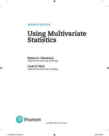
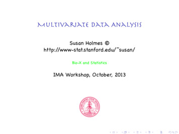
!0.05!0.10.23-Dimensional MDS mapping of legislators based on the 2005U.S. House of Representatives roll call votes. . . . . . . . . . . . . .

!0.05!0.10.23-Dimensional MDS mapping of legislators based on the 2005U.S. House of Representatives roll call votes. Color has beenadded to indicate the party affiliation of each representative. . . . . . . . . . . . . .

Metric Multidimensional ScalingGiven a distance matrix (or its square) how do we find the points inEuclidean space whose distances are given by this matrix?Can we always find such a map?Schoenberg (1935) but also Borschadt 1866.Think of towns, whose road distances are known for whom we wantto reconstruct a map. . . . . . . . . . . . . .

Decomposition of DistancesIf we started with original data in Rp that are not centered: Y,apply the centering matrixX HY,1with H (I 11′ ), and 1′ (1, 1, 1 . . . , 1)nCall B XX′ , if D(2) is the matrix of squared distances betweenrows of X in the euclidean coordinates, we can show that1 HD(2) H B2We can go backwards from a matrix D to X by taking theeigendecomposition of B in much the same way that PCA providesthe best rank r approximation for data by taking the singular valuedecomposition of X, or the eigendecomposition of XX′ . s1 0 0 0 . 0 s2 0 0 . (r)(r) ′(r) X US V with S 0 0 . . . 0 0 . sr . . . . 0 0. . . . . . . . . . . . . .

Multidimensional Scaling also called PCoASimple classical multidimensional scaling. Square D elementwise D(2) D2 . Compute 12 HD2 H B.Diagonalize B to find the principal coordinates.Important: What D to use. . . . . . . . . . . . . .