Transcription
Introduction to R for Multivariate Data AnalysisFernando MiguezJuly 9, 2007email: miguez@uiuc.eduoffice: N-211 Turner Halloffice hours: Wednesday 12pm or by appointment1IntroductionThis material is intended as an introduction to the study of multivariate statisticsand no previous knowledge of the subject or software is assumed. My main objectiveis that you become familiar with the software and by the end of the class you shouldhave an intuitive understanding of the subject. I hope that you also enjoy the learningprocess as much as I do. I believe that for this purpose R and GGobi will be excellentresources. R is free, open source, software for data analysis, graphics and statistics.Although GGobi can be used independently of R, I encourage you to use GGobi as anextension of R. GGobi is a free software for data visualization (www.ggobi.org). Thissoftware is under constant development and it still has occasional problems. However,it has excellent capabilities for learning from big datasets, especially multivariate data.I believe that the best way to learn how to use it is by using it because it is quite userfriendly. A good way of learning GGobi is by reading the book offered on-line andthe GGobi manual, which is also available from the webpage. It is worth saying thatGGobi can be used from R directly by a very simple call once the rggobi packageis installed. In the class we will also show examples in SAS which is the leadingcommercial software for statistics and data management.This manual is a work in progress. I encourage you to read it and provide mewith feedback. Let me know which sections are unclear, where should I expand thecontent, which sections should I remove, etc. If you can contribute in any way it willbe greatly appreciated and we will all benefit in the process. Also, if you want todirectly contribute, you can send me texts and figures and I will be happy to includeit in this manual.Let us get to work now and I hope you have fun!
1.1Installing Rhttp://www.r-project.org/Select a mirror and go to "Download and Install R"These are the steps you need to follow to install R and GGobi.1) Install R.2) type in the command r")3) In this step make sure you install the GTk environment and youbasically just choose all the defaults.4) You install the rggobi package from within R by going toPackages . Install packages . and so on.1.2First session and BasicsWhen R is started a prompt indicates that it is ready to receive input. In a questionand answer manner we can interrogate in different ways and receive an answer. Forexample, one of the simplest tasks in R is to enter an arithmetic expression and receivea result. 5 7[1] 12 # This is the result from RProbably the most important operation in R is the assignment, -. This is usedto create objects and to store information, data or functions in these objects. Anexample:res.1 - 5 7Now we have created a new object, res.1, which has stored the result of thearithmetic operation 5 7. The name res.1 stands for “result 1”, but virtually anyother name could have been used. A note of caution is that there are some conventionsfor naming objects in R. Names for objects can be built from letters, digits and theperiod, as long as the first symbol is not a period or a number. R is case sensitive.Additionally, some names should be avoided because they play a special role. Someexamples are: c, q, t, C, D, F, I, T, diff, df, pt.1.31.3.1Reading and creating data framesCreating a data frameThere are many ways of importing and/or creating data in R. We will look at justtwo of them for simplicity. The following code will prompt a spreadsheet where youcan manually input the data and, if you want, rename columns,2
dat - data.frame(a 0,b 0,c 0)fix(dat)# These numbers should be entered 2 5 4 ; 4 9 5 ; 8 7 9The previous code created an object called dat which contains three columnscalled a, b, and c. This object can now be manipulated as a matrix if all the entriesare numeric (see Matrix operations below).1.3.2Importing dataOne way of indicating the directory where the data file is located is by going to "File"and then to "Change dir.". Here you can browse to the location where you areimporting the data file from. In order to create a data frame we can use the followingcode for the data set COOKIE.txt from the textbook.cook - read.table("COOKIE.txt",header T,sep "",na.strings ".")cook[1:3,]pairs(cook[,5:9])The second line of code selects the first three rows to be printed (the columns werenot specified, so all of them are printed). The header option indicates that the firstrow contains the column names. The sep option indicates that entries are separatedby a space. Comma separated files can be read in this way by indicating a commain the sep option or by using the function read.csv. You can learn more about thisby using help (e.g. ?read.table, ?read.csv). The third line of code produces ascatterplot matrix which contains columns 5 through 9 only. This is a good way ofstarting the exploration of the data.1.4Matrix operationsWe will create a matrix A (R is case sensitive!) using the as.matrix function fromthe data frame dat. The numeral, #, is used to add comments to the code.A - as.matrix(dat)Ap - t(A)ApA - Ap %*% AAinv - solve(A)library(MASS)#####the function t() returns the transpose of Athe function %*% applies matrix multiplicationthe function solve can be used to obtain the inversethe function ginv from the package MASS calculatesa Moore-Penrose generalized inverse of AAginv - ginv(A)Identity - A %*% Ainv # checking the properties of the inverseround(Identity)# use the function round to avoid rounding errorsum(diag(A))# sums the diagonal elements of A; same as tracedet(A)# determinant of ANow we will create two matrices. The first one, A, has two rows and two columns.The second one, B, has two rows and only one column.3
A - matrix(c(9,4,7,2),2,2)B - matrix(c(5,3),2,1)C - A 5D - B*2DDD - A %*% B# matrix multiplicationDDDD - A * A# elementwise multiplicationE - cbind(B,c(7,8))# adds a columnF - rbind(A,c(7,8))# adds a rowdim(A)# dimensions of a matrixO - nrow(A)# number of rowsP - ncol(A)# number of columnsrowSums(A)# sums for each columnMean - colSums(A)/O# mean for each columnFor additional introductory material and further details about the R language see[7].1.5Some important definitionsSome concepts are important for understanding statistics and multivariate statisticsin particular. These will be defined informally here: Random Variable: the technical definition will not be given here but it is important to notice that unlike the common practice with other mathematicalvariables, a random variable cannot be assigned a value; a random variabledoes not describe the actual outcome of a particular experiment, but ratherdescribes the possible, as-yet-undetermined outcomes in terms of real numbers.As a convention we normally use X for a random variable and x as a realizationof that random variable. So x is an actual number even if it is unknown. Expectation: the expectation of a continuous random variable is defined as,ZE(X) µ xf (x)dxYou can think of the expectation as a mean. The integration is done over thedomain of the function, which in the case of the normal goes from to . Mean vector : A mean vector is the elementwise application of the Expectationto a column vector of random variables. E(X) E(X1 )E(X2 ).E(Xp )4 µ1µ2.µp µ
covariance matrix :Σ E(X µ )(X µ)0or Σ Cov(X) 1.6σ11 σ12 · · · σ1pσ21 σ22 · · · σ2p. . .σp1 σp2 · · · σpp Eigenvalues and eigenvectorsIn multivariate data analysis many methods use different types of decompositions withthe aim of describing, or explaining the data matrix (or, more typically the variancecovariance or correlation matrix). Eigenvalues and eigenvectors play an importantrole in the decomposition of a matrix. The definition of these terms and the theorycan be found in the notes or the textbook. Here we will see the functions in R usedto carry out these computations. Try the following,A - matrix(c(1,1,0,3),2,2)eigen(A)dm - scan()# Insert 13 -4 2 -4 13 -2 2 -2 10B - matrix(dm,3,3)eigen(B)C - edit(data.frame())# enter these numbers1615201061510610875106189815Cm - as.matrix(C)# coerce the data frame into a matrixmean(Cm)# mean vectorvar(Cm)# variance-covariance matrixcor(Cm)# correlation matrix1.7DistanceThe concept of distance can be defined as a spatial difference between two points.So, in a general sense distance is a difference, and it is a more abstract conceptthat mere spatial difference. For example, we could be interested in the difference inweight of two items. Some methods in this class will involve distance between points in5
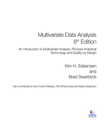
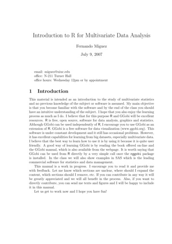
multidimensional space. Most datasets involve variables that suggest spatial distance,others temporal distance and some might not imply a distance that can be measuredquantitatively. These later variables are usually named categorical (or classification)variables.More formally, if we consider the point P (x1 , x2 ) in the plane, the Euclideandistance, d(O, P ), from P to the origin O (0, 0) is, according to the Pythagoreantheorem,qd(O, P ) x21 x21(1)In general if the point P has p coordinates so that P (x1 , x2 , . . . , xp ), the Euclideandistance from P to the origin O (0, 0, . . . , 0) isqd(O, P ) x21 x22 · · · x2p(2)All points (x1 , x2 , . . . , xp ) that lie a constant squared distance, such as c2 , fromthe origin satisfy the equationd2 (O, P ) x21 x22 · · · x2p c2(3)Because this is the equation of a hypershpere (a circle if p 2), points equidistantfrom the origin lie on a hypershpere. The Euclidean distance between two arbitrarypoints P and Q with coordinates P (x1 , x2 , . . . , xp ) and Q (y1 , y2 , . . . , yp ) is givenbyqd(P, Q) (x1 y1 )2 (x2 y2 )2 . . . (xp yp )2(4)This measure of distance is not enough for most statistical methods. It is necessary, therefore, to find a ‘statistical’ measure of distance. Later we will see themultivariate normal distribution and interpret the statistical distance in that context.For further details about this section see [5].1.8Univariate graphics and summariesA good way of exploring data is by using graphics complemented by numerical summaries. For example, we can obtain summaries for columns 5 through 9 from theCOOKIE data sity(cook[,5]))# 5 numbers summary# boxplots for 5 variables# density plot for variables in column 5At this point it is clear that for a large dataset, this type of univariate exploration isonly marginally useful and we should probably look at the data with more powerfulgraphical approaches. For this, I suggest turning to a different software: GGobi.While GGobi is useful for data exploration, R is preferred for performing the numericalpart of multivariate data analysis.6
121086420CELLSIZE CELLUNIF SURF ROLOOSEFIRMFigure 1: Boxplots for 5 variables in COOKIE dataset7
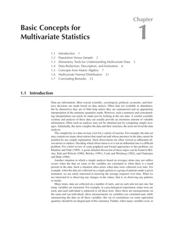
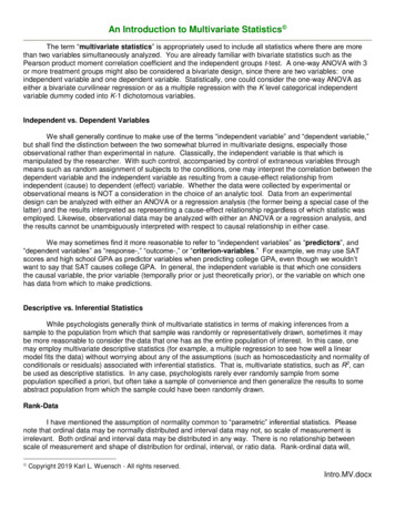
2Multivariate data setsTypical multivariate data sets can be arranged into a data matrix with rows andcolumns. The rows indicate ‘experimental units’, ‘subjects’ or ‘individuals’, whichwill be referred as units from now on. This terminology can be applied to animals,plants, human subjects, places, etc. The columns are typically the variables measuredon the units. For most of the multivariate methods treated here we assume that thesevariables are continuous and it is also often convenient to assume that they behaveas random events from a normal distribution. For mathematical purpose, we arrangethe information in a matrix, X, of N rows and p columns, x11 x12 · · · x1p x21 x22 · · · x2p X . . ···. xN 1 xN 2 · · · xN pwhere N is the total number of ‘units’, p is the total number of variables, and xijdenotes the entry of the j th variable on the ith unit. In R you can find example datasets that are arranged in this way. For example,dim(iris)[1] 150 21.41.5SpeciessetosaversicolorvirginicaWe have asked R how many dimensions the iris dataset has using the dim function. The dataset has 150 rows and 5 columns. The rows are the experimental units,which in this case are plants. The first four columns are the response variables measured on the plants and the last column is the Species. The next command requestsprinting rows 1,51 and 120. Each of these is an example of the three species in thedataset. A nice visual approach to explore this dataset is the pairs command, whichproduces Figure 2. The code needed to produce this plot can be found in R by typing?pairs. Investigate!3Multivariate Normal DensityMany real world problems fall naturally within the framework of normal theory. Theimportance of the normal distribution rests on its dual role as both population modelfor certain natural phenomena and approximate sampling distribution for many statistics [5].8
Anderson's Iris Data 3 species2.03.04.0 2.5 1.50.5 5.5 Petal.Length 7.5 1234567Figure 2: Scatterplot matrix for iris dataset97.5 2.5 6.5 4.5Sepal.Width 1.56.5 0.55.54.04.5Sepal.Length3.0Petal.Width1 2 3 4 5 6 72.0
3.1The multivariate Normal Density and its PropertiesThe univariate normal is a probability density function which completely determinedby two familiar parameters, the mean µ and the variance σ 2 ,f (x) 1exp [(x µ)/σ]2 /2 x 2πσ 2The term in the exponent 2x µ (x µ)(σ 2 ) 1 (x µ)σof the univariate normal density function measures the square of the distance fromx to µ in standard deviation units. This can be generalized for a p 1 vector x ofobservations on several variables as(x µ)0 Σ 1 (x µ)The p 1 vector µ represents the expected value of the random vector X, andthe p p matrix Σ is the varaince-covariance matrix of X. Given that the symmetricmatrix Σ is positive definite the previous expression is the square of the generalized distance from x to µ. The univariate normal density can be generalized to ap dimensional normal density for the random vector X0 [X1 , X2 , . . . , Xp ]f (x) 0 11exp (x µ) Σ (x µ)/2(2π)p/2 Σ 1/2where xi , i 1, 2, . . . , p. This p dimensional normal density isdenoted by Np (µ, Σ).3.2Interpretation of statistical distanceWhen X is distributed as Np (µ, Σ),(x µ)0 Σ 1 (x µ)is the squared statistical distance from X to the population mean vector µ. Ifone component has much larger variance than another, it will contribute less to thesquared distance. Moreover, two highly correlated random variables will contributeless than two variables that nearly uncorrelated. Essentially, the use of the inverseof the correlation matrix, (1) standardaizes all of the variables and (2) eliminates theeffects of correlation [5].3.3Assessing the Assumption of NormalityIt is important to detect moderate or extreme departures from what is expectedunder multivariate normality. Let us load the Cocodrile data into R and investigatemultivariate normality. I will select variables sl through wn to keep the size of theindividual scatter plots informative.10
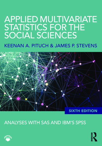
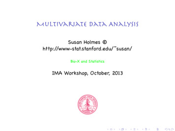
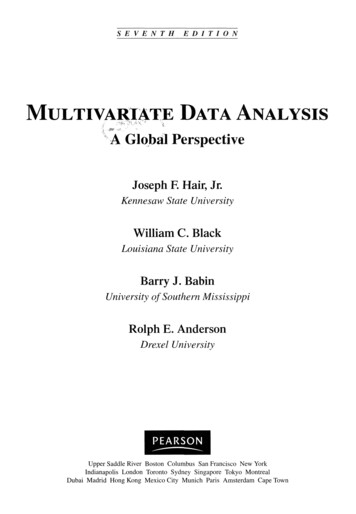
Croco - read.csv("Cocodrile.csv", header T, na.strings ".")names(Croco)[1] "id""Species" "cl""cw""sw""sl"[8] "ow""iow""ol""lcr""wcr""wn"pairs(Croco[,6:13])100 500 dcl 20 60 8020 50 100400 10 60 2060100 400100 wcr lcr 70 40 10 ol 40 20 100 60 iow ow 20 50 6020sl 20 20 60 50 150100 400 700"dcl" 50wn150Figure 3: Scatterplot matrix for Cocodrile datasetThis data set is probably too clean, but it is a good first example where we seethe high degree of correlation among the variables and it seems plausible to assumebivariate normality in each one of the plots and therefore multivariate normality forthe data set in general. Let us turn to another example using the Skull.csv data set.We can basically follow the same steps as we did for the first dataset. The resultingscatterplot matrix reveals the unusually high correlation between BT and BT1. BT1is a corrected version of BT and therefore we should include only one of them in theanalysis.11
130 120 140 8595105 BL1 115Figure 4: Scatterplot matrix for Skull dataset12 BL 60100 140 BH 60 120130140 55MB 120 130 140 115 140105 80 100956085140NH501304512045505560
4Principal Components AnalysisPrincipal component analysis (PCA) tries to explain the variance-covariance structureof a set of variables through a few linear combinations of these variables [2]. Itsgeneral objectives are: data reduction and interpretation. Principal components isoften more effective in summarizing the variability in a set of variables when thesevariables are highly correlated. If in general the correlations are low, PCA will beless useful. Also, PCA is normally an intermediate step in the data analysis sincethe new variables created (the predictions) can be used in subsequent analysis suchas multivariate regression and cluster analysis. It is important to point out that thenew variables produced will be uncorrelated.The basic aim of principal components analysis is to describe the variation in a setof correlated variables, x1 , x2 , . . . , xp , in terms of a new set of uncorrelated variablesy1 , y2 , y3 , . . . , yp , each of which is a linear combination of the x variables. The newvariables are derived in increasing order of “importance” in the sense that y1 accountsfor as much of the variation in the original data amongst all linear combinations ofx1 , x2 , . . . , xp . Then y2 is chosen to account for as much as possible of the remainingvariation, subject to being uncorrelated with y1 and so on. The new variables definedby this process, y1 , y2 , . . . , yp are the principal components.The general hope of principal components analysis is that the first few componentswill account for a substantial proportion of the variation in the original variables andcan, consequently, be used to provide a convenient lower-dimensional summary ofthese variables that might prove useful in themselves or as inputs to subsequentanalysis.4.1Principal Components using only two variablesTo illustrate PCA we can first perform this analysis on just two variables. For thispurpose we will use the crabs dataset.crabs - read.csv("australian-crabs.csv",header T)Select variables "FL" and "RW".crabs.FL.RW - crabs[c("FL","RW")]Scale (or standardize ) variables. This is convenient for latter computations.crabs.FL.RW.s - scale(crabs.FL.RW)Calculate the eigenvalues and eigenvectors.eigen(cor.crabs) values[1] 1.90698762 0.09301238 vectors[,1][,2][1,] 0.7071068 0.7071068[2,] 0.7071068 -0.707106813
Following we will analyze the APLICAN data in R, which is also analyzed in theclass textbook.appli - read.table("APPLICAN.txt",header T,sep "")colnames(appli) - "EXP","DRV","AMB","GSP","POT","KJ","SUIT")First I added the column names as this was not supplied in the original dataset.dim(appli)[1] 48 16(appli.pc - princomp(appli[,2:16]))summary(appli.pc)Compare the output from R with the results in the book. Notice that R does notproduce a lot of output (this is true in general and I like it). The “components” arealso standard deviations and they are the squared root of the Eigenvalues that yousee in the textbook. Let’s do a little of R gymnastics to get the same numbers as thebook.appli.pc sdev 2Comp.1Comp.2Comp.366.1420263 18.1776339 37661I’m showing only the first 6 components here. With the summary method we canobtain the Proportion and Cumulative shown on page 104 in the text book. TheSCREE plot can be obtain using the plot function. The loadings function will giveyou the output on page 105.This is a good oportunity to use GGobi from R.library(rggobi)ggobi(appli)55.1Factor AnalysisFactor Analysis ModelLet x be a p by 1 random vector with mean vector µ and variance-covariance matrixΣ. Suppose the interrelationships between the elements of x can be explained by thefactor modelx µ Λf ηwhere f is a random vector of order k by 1 (k p), with the elements f1 , . . . , fk ,which are called the common factors; Λ is a p by k matrix of unknown constants,called factor loadings; and the elements, η1 , . . . , ηp of the p by 1 random vector η are14
mp.7Comp.9Figure 5: SCREE plot of the eigen values for APPLICAN dataset15
called the specific factors. It is assumed that the vectors f and η are uncorrelated.Notice that this model resembles the classic regression model with the difference thatΛ is unknown.The assumptions of this model can be summarized1. f (0, I)2. η (0, Ψ), where Ψ diag(ψ1 , . . . , ψp ) and3. f and η are independent.The assumptions of the model then lead toΣ LL0 ΨUnder this model the communalities and more generally the factorization of Σremain invariant of an orthogonal transformation. Hence, the factor loadings aredetermined only up to an orthogonal transformation [4].5.2Tests exampleBefore I introduce an example in R let me say that different software not only producedifferent results because they might be using different methods but they even producevery different results using apparently the same method. So it should be of no surpriseif you compare the results from this analysis with SAS, SPSS, SYSTAT and you seelarge differences.This is an example I made up and it is based on tests that were taken by 100individuals in arithmetic, geometry, algebra, 200m run, 100m swim and 50m run.First we create the object based on the data test - read.table("MandPh.txt",header T,sep "") names(test)[1] "Arith" "Geom" "Alge" "m200R" "m100S" "m50R"The correlation matrix is round(cor(test),2)Arith Geom Alge m200R m100S m50RArith 1.00 0.88 0.78 0.19 0.24 0.25Geom0.88 1.00 0.90 0.16 0.18 0.18Alge0.78 0.90 1.00 0.19 0.20 0.20m200R 0.19 0.16 0.19 1.00 0.90 0.78m100S 0.24 0.18 0.20 0.90 1.00 0.89m50R0.25 0.18 0.20 0.78 0.89 1.0016
This matrix clearly shows that the ‘math’ tests are correlated with each other andthe ‘physical’ tests are correlated with each other, but there is a very small correlationbetween any of the ‘math’ and the ‘physical’.There are different ways of entering the data for factor analysis. In this casewe will just use the object we created in the first step. The only method in R forconducting factor analysis is maximum likelihood and the only rotation available is“varimax”. test.fa1 - factanal(test, factor 1) test.fa1.Test of the hypothesis that 1 factor is sufficient.The chi square statistic is 306.91 on 9 degrees of freedom.The p-value is 8.91e-61 test.fa2 - factanal(test, factor 2).Test of the hypothesis that 2 factors are sufficient.The chi square statistic is 5.2 on 4 degrees of freedom.The p-value is 0.267The fact that we do not reject the null hypothesis with two factors indicates thattwo factors are needed and this makes sense considering the way we generated thedata. We can store the loadings in an object called Lambda.hat and the uniquenessin an object called Psi.hat and recreate the correlation matrix. Lambda.hat - test.fa2 loadingsPsi.hat - diag(test.fa2 uni)Sigma.hat - Lambda.hat%*%t(Lambda.hat) Psi.hatSigma.hatround(Sigma.hat,2)Arith Geom Alge m200R m100S m50RArith 1.00 0.88 0.80 0.21 0.24 0.23Geom0.88 1.00 0.90 0.16 0.18 0.18Alge0.80 0.90 1.00 0.18 0.20 0.19m200R 0.21 0.16 0.18 1.00 0.90 0.80m100S 0.24 0.18 0.20 0.90 1.00 0.89m50R0.23 0.18 0.19 0.80 0.89 1.00Notice that in this case Sigma.hat is really the fitted correlation matrix and itdiffers slightly from the original. This difference is the “lack of fit” which will be seenin more detail in the next example.5.3Grain exampleThis examples was taken from a book by Khattree and Naik (1999).17
Sinha and Lee (1970) considered a study from agricultural ecology where composite samples of wheat, oats, barley, and rye from various locations in the Canadianprairie were taken. Samples were from commercial and governmental terminal elevators at Thunder Bay (Ontario) during the unloading of railway boxcars. The objectiveof the study was to determine the
Introduction to R for Multivariate Data Analysis Fernando Miguez July 9, 2007 email: miguez@uiuc.edu office: N-211 Turner Hall office hours: Wednesday 12pm or by appointment 1 Introduction This material is intended as an introduction to the study of multivariate statistics and no previous kno