Transcription
Regression analysis in practice with GRETLPrerequisitesYou will need the GNU econometrics software GRETL installed on your computer(http://gretl.sourceforge.net/), together with the sample files that can be installed fromhttp://gretl.sourceforge.net/gretl data.html.This is no econometrics textbook, hence you should have already read some econometrics text, suchas Gujarati’s Basic Econometrics (my favorite choice for those with humanities or social sciencebackground) or Greene’s Econometric Methods (for those with at least BSc in Math or relatedscience).1. Introduction to GRETL1.1 Opening a sample file in GRETLNow we open data3-1 of the Ramanathan book (Introductory econometrics wit applications, 5th ed.).You can access the sample files in the File menu under Open data/Sample file Once you click on the sample files you are shown a window with the sample files installed on yourcomputer. The sheets are named after the author of the textbook which the sample files are takenfrom.
Choose the sheet named “Ramantahan” and choose data3-1.You can open the dataset by left-clicking on its name twice, but if you right click on it, you will havethe option to read the metadata (info).This may prove useful because sometime it gives you the owner of the data (if it was used for anarticle), and the measurement units and exact description of the variables.
1.2 Basic statistics and graphs in GRETLWe have now our variables with descriptions in the main window.You can access to basic statistics and graphs my selecting one (or more by holding down ctrl) of thevariables by right-click.
Summary statistics will yield you the expected statistics.Frequency distribution should give you a histogram, but first you need to choose the number of bins.With 14 observations 5 bins look enough.You also have a more alphanumerical version giving you the same information:
You also ask for a boxplot.Showing that the prices are skewed to the right (the typical price being less than the average) whichis often referred to as positive skew.If you choose both variables, you have different options as they are now treated as a group ofpossibly related variables.The option scatterplot will give you the following:
Which already shows that a linear relationship can be assumed between the price of houses andtheir area. A graphical analysis may be useful as long as you have a two-variate problem. If you havemore than two variables, such plots are not easy to understand anymore, so you should rely on 2Drepresentation of problems like different residual plots.You can also have the correlation coefficient estimated between the two variables:With a hypothesis test with the null hypothesis that the two variables are linearly independent oruncorrelated. This is rejected at a very low level of significance (check out the p-value: it is muchlower than any traditional level of significance, like 0.05 (0.01) or 5% (1%)).1.3 transforming variablesTransforming variables can be very useful in regression analysis. Fortunately, this is very easily donein GRETL. You simple choose the variables that you wish to transform and choose the Add menu. Themost often required transformations are listed (the time-series transformations are now inactivesince our data is cross-sectional), but you can always do you own transformation by choosing “Definenew variable” .
Let us transform our price into a natural logarithm of prices. This is done by first selecting price, thenby left-clicking the Logs of selected variables in the Add menu. You will now have the transformedprice variable in you main window as well.Now that you know the basics of GRETL, we can head to the first regression.2. First linear regression in GRETL2.1 Two-variate regressionYou can estimate a linear regression equation by OLS in the Model menu:
By choosing the Ordinary Least Squares you get a window where you can assign the dependent andexplanatory variables. Let our first specification be a linear relationship between price and area:After left-clicking OK, we obtain the regression output:
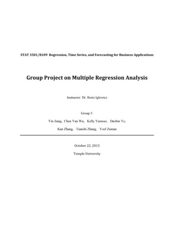
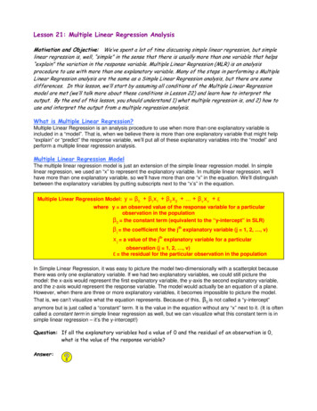
The intercept does not seem to be statistically significant (i.e. the population parameter is notdifferent from zero at 10% level of significance), while the slope parameter (the coefficient of thearea) is significant at even 1%. The R2 is also quite high (0.82) signifying a strong positive relationshipbetween the area of houses and their prices. If a house had one square feet larger living area, its saleprice was on average higher by 138.75 dollar.2.2 Diagnostic checks -heteroscedasticityBut this does not mean that we should necessarily believe our results. The OLS is BLUE (BestUnbiased Linear Estimator) only if the assumptions of the classical linear model are fulfilled. Wecannot test for exogeneity (that is difficult to test statistically anyway), and since we have crosssectional data, we should also not care much about serial correlation. We can test heteroscedasticityof the residual though. Heteroscedasticity means that the variance of the error is not constant. Fromestimation point of view what really matters is that the residual variance should not be dependenton the explanatory variables. Let us look at this graphically. Go to the Graph menu in the regressionoutput.Plotting the residuals against the explanatory variable will yield:
You can observe that while the average of the residual is always zero, its spread around its meandoes seem to depend on the area. This is an indication of heteroscedasticity. A more formal test is aregression of the square of the residuals on the explanatory variable(s). This is the Breusch-Pagantest:What you obtain after clicking on the Breush-Pagan test under Tests menu is the output of the testregression. You can observe that the squared residuals seem to depend positively on the value ofarea, so the prices of larger houses seem to have a larger variance than those of smaller houses. Thisis not surprising, and as you can see, heteroscedasticity is not an error but rather a characteristic ofthe data itself. The model seems to perform better for small houses than for bigger ones.
You can also check the normality of the residuals under the Tests menu:Even though normality itself is not a crucial assumption, with only 14 observations we cannot expectthat the distribution of the coefficients is close to normal unless the dependent variable (and theresidual) follows a normal distribution. Hence this is a good news.Heteroscedasticity is a problem though inasmuch as it may affect the standard errors of thecoefficients, and may reduce efficiency. There are two solutions. One is to use OLS (since it is stillunbiased), but have the standard errors corrected for heteroscedasticity. This you can achieve byreporting heteroscedasticity robust standard errors, which is the popular solution. Go back to theModel menu, and OLS, and have now robust standard errors selected:
While the coefficients did not change, the standard errors and the t-statistics did.An alternative way is to transform you data so that the homoscedasticity assumption becomes validagain. This requires that observation with higher residual variance are given lower weight, whileobservations where the residual variance was lower are given a relatively higher weight. Theresulting methodology is called the Weighted Least Squares (WLS) or sometime it is also referred tothe Feasible Generalized Least Squares (FGLS). You can achieve this option in the Model menu under“Other linear models” as “heteroscedasticity corrected”.
You may wonder which one is better? To transform your data or rather to have only you standarderrors corrected and stick with the OLS. You can see that there may be significant changes in the tstatistics, while the coefficients are basically the same. Hence it is often the case that you do not gainmuch by reweighting your data. Nevertheless, theoretically both are correct ways to treatheteroscedasticity. The majority of articles report robust statistics and does not do WLS, partly forconvenience, and partly because there is some degree of distrust toward data that has been altered:do not forget that once you weight your data it is not the same data anymore, but, in this particularcase, all your variables (including the dependent variable) will be divided by the estimated standarderror of the residual for that particular observation.2.3 Alternative specificationsWe may also try a different specification: since the prices are skewwed to the right, a logartihmictransformation may just bring it more to the center. For a visuals look of the idea, let us look at thehistogram of log prices.Indeed it look much more centered than prices. This may have improving effects on the model, eventhough there is no guarantee. We need to estimate the alternative model and compare it with theoriginal one.
We obtain now a statistically significant constant term, saying that a building with null area wouldsell at exp(4.9) 134.3 thousands dollar (this is a case when the constant seemingly has no deepeconomic meaning, even though you may say that this is the price of location, or effect of fixed costfactors on price), and every square feet additional area would increase the price by 0.04% on average(do not forget to multiply by 100% if log is in the left-hand side). You may be tempted to say that thislog-lin (or exponential) specification is better than the linear specification, simply, because its R 2exceeds that of the original specification. This would be a mistake though. All goodness of fitstatistics, including R2, the log-likelihood, or the information criteria (Akaike, Schwarz and HannanQuinn) are dependent on the measurement unit of the dependent variable. Hence, if the dependentvariable does not remain the same, you cannot use these for a comparison. They can only be utilizedfor model selection (i.e. telling which specification describes the dependent variable better) if theleft-hand side of the regression remains the same, albeit you can change the right-hand side as youplease.In such situations when the dependent variable has been transformed, the right way to comparedifferent models is to transform the fitted values (as estimated from the model) to the same units asthe original dependent variable, and look at the correlation between the original variable and thefitted values from the different specifications. Hence, now, we should save the fitted values from thisregression, than take its exponential, so that it is in thousand dollars again, and look at thecorrelation with the dependent variable. Saving the fitted values is easy in GRETL:
Let us call the fitted values lnpricefitexp:Now we have the fitted values from the exponential model as a new variable. Let us take theexponential of it:
Let us also save the fitted values from the linear model as pricefitlinear. We can now estimate thecorrelations:We can observe that the linear correlation coefficient between price and the fitted price from thelinear model is 0.9058, while the correlation between the price and the fitted price from theexponential specification is 0.8875. Hence the linear model seems better.
3.Multivariate regression3.1 Some important motivations behind multivariate regressionsLife is not two-dimensional so two-variate regression are rarely useful. We need to continue into therealm of multivariate regressions.As you have seen in the lecture notes on OLS, multivariate regressions has the great advantage thatthe coefficients of the explanatory variables can be interpreted as net or ceteris paribus effects. Inother words, the coefficient of variable x can be seen as the effect of x on the dependent variable ywith all other explanatory variables fixed. This is similar to the way of thinking behind comparativestatics. But beware! This is only true for variables which are included in the regression. If you omitvariables that are important and correlated with the variables that you actually included in yourregression, the coefficients will reflect the effect of the omitted variable too. Let us take the twovariate regression from section 2 as an example. It is quite obvious that house prices depend not onlyon the area of houses, but also on the quality of buildings, their distance from the city centre, or thenumber of rooms, etc. By including the area only as explanatory variable, you do not really measurethe effect of area on the sale prices, but rather the total effect of area, including part of the effect ofother factors that are not in your model but are related to area. If, for example, bigger houses areusually farther from the city centre, then the coefficient of the area will not only reflect that biggerhouses are more valuable, but also that bigger houses are further away from the centre and hencetheir prices should be somewhat lowered because of this. The total effect of area on house pricesshould then be lower than the net effect, which would be free of the distance effect). You canobserve this simply, by introducing new variables into a specification. You will have a big chance thatimportant additional explanatory variables will change the coefficient of other explanatory variables.Be therefore very well aware of the problem of omitted variables and the resulting bias. You can onlyinterpret a coefficient as the net effect of that particular factor, if you have included all importantvariables in your regression, or you somehow removed the effect of those omitted variables (panelanalysis may offer that).3.2 Estimating a Mincer equationWe need now a different sample file: open wage2 of the Wooldridge datafiles.You will find observations on socio-economic characteristics of 526 employees. The task is to find outhow these characteristics affect their wages. These type of models are called Mincer equation, afterJacob Mincer’s empirical work. The basic specification is as follows:kln wagei 0 1educi j X ji uij 2where the coefficient of the education (usually but not exclusively expressed as years of education) isthe rate of returns to education, and X denote a number of other important variables affecting wagesuch as gender, experience, race, job category, or geographical position.Let us estimate the coefficient with all available variables.
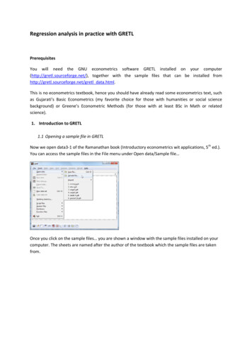
What we find is a reasonable R2, and a lot of statistically insignificant variables. We will discuss howto reduce our model later, but let us first review the interpretation of the coefficients.Since we have log wages on the left-hand side, the effect of explanatory variables should beinterpreted as relative effects. For example the educ coefficient is 0.047, that is, if we have twoemployees who has the same gender, work in the same field, has the same experience and work attheir present employer for the same time, the one with one year more education will have 4.7%higher salary on average. The female dummy is statistically significant and negative -0.268. Theinterpretation is, that if all other factors are the same, being woman will cause the wage to be exp(0.268)-1 -0.235, that is 23.5% lower than for a man. We do not find a comparable result for race.Another interesting feature of the model is the presence of squared explanatory variables, orquadratic function forms. You can see that it is not only experience that is included but also itssquare. This functional form is often used to capture non-linearities, i.e., when the effect of anexplanatory variable depends on its own values as well. For example, there is reason to believe thatexperience has a large effect on wages initially, but at later phases this effect fades away. This issimply because the first few years are crucial to learn all those skills that are necessary for you to bean effective employee, but once you have acquired those skills, your efficiency will not improve muchsimply by doing the same thing for a longer time. This is what we find here as well. The positivecoefficient of the experience suggests that at low levels of experience, any further years have a
positive impact on wages (2.5% in the first year), but this diminishes as shown by the squaredexperience. If we have a specification as follows:yi 0 1 xi 2 xi2 ui then the marginal effect of x can be calculated as follows.dy 1 2 2 xidxWe can use above expression to plot a relationship between the effect of experience on wage andexperience:3.0%2.5%2.0%1.5%1.0%0.5%0.0%-0.5% 01020experience (years)304050-1.0%-1.5%-2.0%After a while, it may even be that the effect of experience is negative in the wage, even though thismay simple be because we force a quadratic relationship onto out data.3.3 Model selectionShould we or should we not omit the variables that are not significant at at least 10%? This is aquestion that is not easy to answer.Statistically speaking, if we include variables that are not important (their coefficients are statisticallynot significant) we will still have unbiased results, but the efficiency of the OLS estimator will reduce.Hence, we can have that by including non-essential variables in our regression, an important variablewill look statistically insignificant. Hence purely statistically speaking removing insignificant variablesis a good idea. Yet, very often you will find that insignificant coefficients are still reported. The reasonis that sometimes having a particular coefficient statistically insignificant is a result by its own right,or the author wishes to show that the results are not simply due to omitted variable bias, and henceleave even insignificant variables in the specification to convince the referees (who decide if anarticle is published or not). It may be a good idea though to report the original (or unrestricted)specification and a reduced (or restricted) specification as well.But which way is the best? Should you start out with a single explanatory variable and keep addingnew variables, or rather should you start with the most complex model, and reduce it by removing
insignificant variables until you have all variables statistically significant. This question can beanswered very simply. It should be the second way. Do not forget, that having unnecessary variablesdoes not cause a bias in your parameter estimates, while omitting important variables does. Hence ifyou start out with single variable, you statistics on which you base your decision if you should add orremove a variable will be biased too. Having less efficient but unbiased estimates is now the lesserbad.The standard method is to reduce you model by a single variable in each step. It is logical to removethe variable with the highest p-value. The process can also be automatized such as in GRETL. Theomit variables option in the Tests menu allows you to choose automatic removal of variables.This option allows you to assign the p-value at which a variables should be kept in the specification.Choosing this value 0.10 means that only variables that are significant at at least 10% will be retainedin the specification.
The resulting specification is:
3. Multivariate regression 3.1 Some important motivations behind multivariate regressions Life is not two-dimensional so two-variate regression are rarely useful. We need to continue into the realm of multivariate regressions. As you have seen in the lecture notes on OLS, multivariate regressions has the great advantage that