WIXLIB

Multivariate Time Series Analysis in RRuey S. TsayBooth School of BusinessUniversity of ChicagoMay 2013, R/Finance Conference

ObjectiveAnalysis of multivariate time-series data using R:ITo obtain parsimonious models for estimationITo extract “useful” information when the dimension is highITo make use of prior information or substantive theoryITo consider also multivariate volatility modeling andapplications

Outline (3 main parts)IMultivariate time series analysis (”MTS” package)1. VAR, VMA, VARMA, Seasonal VARMA, VARMAX, Factormodels, Multivariate volatility models, etc.2. Simple demonstrationIFactor models (dimension reduction)1.2.3.4.IConstrained factor modelsA motivating examplePartially constrained factor modelsApplication in risk managementPrincipal volatility component analysis1. Generalized kurtosis matrix2. Simple illustration

Multivariate time series analysisIDifficulties1. Too many parameters when the dimension is high2. Identifiability problemsISolutions1. Stay away: focus on Vector autoregressive models (VAR)2. Structural specification: Kronecker index and ScalarcomponentsTools used: Canonical correlation analysis, likelihood ratio test3. Factor models (with or without constraints)Tools used: PCA, LASSO, K means, model-based classification

A 2-dimensional VARMA(2,2) model zt 0.6 0.5 0.1 0.3 zt 1 zt 2 0.5 0.60.3 0.1 1.05 0.15 0.26 0.06 at at 1 at 2 ,0.15 1.050.06 0.26where Cov(at ) Σa 0.The model can be simplified! wt z1t z2t satisfies(1 0.5B)wt (1 0.5B)bt .

10 0 10z1t0100020003000400050006000400050006000 10 0 10z2ttime0100020003000timeFigure: Simulation: a bivariate series with 6000 observations

Model specificationIVAR models1. AIC and HQ: VAR(12)2. BIC: VAR(10)3. Tiao-Box chi-square: VAR(13)IVARMA models1. ECCM (Tiao-Tsay): VARMA(2,2)2. Kronecker index: {2, 1}, implying a VARMA(2,2) model, butwith a VARMA(1,1) component.

e: Time plots of the monthly unemployment rates of the 50 Statesin the U.S. from January 1976 to September 2011. The data areseasonally adjusted.

105rate15Unemployment rates: blk(IL), r(WI), b(MI)19751980198519901995200020052010yearFigure: Time plots of the monthly unemployment rates of IL, WI, and MIfrom January 1976 to September 2011. The data are seasonally adjusted.

Summary of modelingIVAR approach: AIC selects a VAR(7) model,with 35 parametersIVARMA approach: a VARMA(2,2) model,with 29 parametersBoth models fit the data reasonably well. The two models aresimilar.

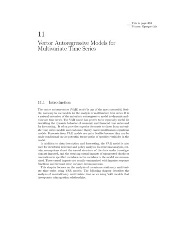
4681224680 2 4IRF* * * * * ** * * * * * *012** * * ** * ** ** * *0246812Orig. innovationsOrig. innovations* * * * * * * * * ** * *246812* * * * * * * * * * * * *024680 2 4Orig. innovationsIRFlag0 2 4lag12** *0* * * * ** * ** *246812Orig. innovationsOrig. innovationsOrig. innovations* * * * * * * ** * * **0246lag812* * * * * * * ** * * * *0246lag8120 2 4lagIRFlag0 2 4lagIRF0 2 42Orig. innovationslag0IRF* * * ** * ** ** *IRF0 2 4IRF0*0 2 4*Orig. innovationsIRF0 2 4IRFOrig. innovations*0**2** * * * * * ** *468lagFigure: Impulse response functions of A VAR(7) model for monthlyunemployment rates of IL, WI, and MI from January 1976 to September2011.12

468122468 1 1 3 5IRF* * * * * * * * * * * * *012* * * ** * ** ** * * *0246812Orig. innovationsOrig. innovations* * * * * * * * * * ** *246812* * * * * * * * * * * * *02468 1 1 3 5Orig. innovationsIRFlag 1 1 3 5lag12* * * * ** * ** ** * *0246812Orig. innovationsOrig. innovationsOrig. innovations* * * * * * * * * * * * *0246lag812* * * * * * * * * * * * *0246lag812 1 1 3 5lagIRFlag 1 1 3 5lagIRF 1 1 3 52Orig. innovationslag0IRF* * * * ** * ** * *IRF 1 1 3 5IRF0* 1 1 3 5*Orig. innovationsIRF 1 1 3 5IRFOrig. innovations*0**2* ** * * ** ** *468lagFigure: Impulse response functions of a VARMA(2,2) model for monthlyunemployment rates of IL, WI, and MI from January 1976 to September2011.12

Factor modelsFor high-dimensional series: Dimension reduction and ease ininterpretation

Approximate factor modelsxt Lf t tyt h β 0 f t γ 0 wt vt hwhere xt is an N-dimensional random vector, L is an N r loadingmatrix, f t is the r -dimensional common factors, wt is apre-determined vector that may contain lagged values of yt , h 0is the forecast horizon, t and vt are the noise terms, respectively.Usual assumptions:I All variables have zero means.I E (f t f 0t ) Ir .I E ( t 0t ) Ψ (positive definite)I E (f t 0t ) 0, E (f t vt h ) 0, & E (wt vt h ) 0.I Rank(L) r and 1 L0 L positive definite as N .NI Additional conditions needed if Ψ is not diagonal, i.e.bounded eigenvalues.

DiscussionsSome difficulties often encountered when N is large:IHard to understand or interpret the estimated commonfactors.IDoes a large N produce more accurate forecasts? (Notnecessarily)Iyt plays no role in factor estimation.IDoes not make use of any prior information or theory or pastexperience.Our goal is to overcome some of these weaknesses.

Constrained factor modelH is an N m matrix of known constraints. The model becomesxt Hωf t twhere ω is an m r matrix, Rank(H) m and Rank(ω) r .Typically, r m N. [Simply put, L Hω.]Examples:IFor stock returns, columns of H may indicate the industrialsectors of the stock.IFor interest rates, columns H may indicate level, slope andcurvature of the yield curve.

Motivating exampleMonthly excess returns of 10 stocks: (less 3-month T bill)(a) Pharmaceutial: Abbott Labs, Eli Lilly, Merck, and Pfizer(b) Auto: General Motors and Ford(c) Oil: BP, Chevron, Royal Dutch, and Exxon-MobilSample period: January 1990 to December 2003 for 168observations.

Example continued: traditional factorsResults of traditional PCA using correlations:IEig. Values: 3.890, 1.971, 1.498, 0.586, 0.498, ., 0.242Ifirst 3 .04620.1115-0.6311-0.70300.19770.13180.13660.0574

Example continued.Make use of the knowledge of three 1 1 1 1 0H0 0 0 0 0 10 0 0 0 0industries: 0 0 0 0 01 0 0 0 0 .0 1 1 1 1Perform a constrained analysis: (least-squares estimates)Eigen Values:IConstrained space: 3.813, 1.917, 1.362IResidual space: 0.660, 0.575, 0.517, ., 0.256.

Example continued: Loading 0.551 -0.497 0.1410.480 -0.649 0.0130.583 -0.605 0.0540.663 -0.471 0.1310.490 0.009 -0.7440.353 0.098 -0.8290.690 0.457 0.2330.739 0.485 0.1550.809 0.342 0.1610.715 0.365 0.068ConstrainedHω0.568 -0.556 0.0740.568 -0.556 0.0740.568 -0.556 0.0740.568 -0.556 0.0740.423 0.071 -0.7830.423 0.071 -0.7830.736 0.409 0.1680.736 0.409 0.1680.736 0.409 0.1680.736 0.409 0.168

Example continued.Discussions:IConstrained model is more parsimonious (10 3 vs. 3 3)ISector variations explain the variability in the excess returns(equal loading for stocks in the same industry)IThe spaces spanned by the common factors are essentially thesame with/without constraintsCanonical correlations between the two sets of commonfactors are0.9997, 0.9990, 0.9952.IBoth maximum likelihood and least squares estimationsavailableITest is available for checking the constraints. Tsai and Tsay(2010, JASA)

Partially constrained factor modelsIn practice, it is likely that only partial constraints are available.xt Hωf t Lgt t ,yt h β 01 f t β 02 gt vt h ,t 1, . . . , T ,where L is an N p unconstrained loading matrix of rank p and gtis a p-dimensional unconstrained common factors.Additional assumptions:E (gt ) 0, E (gt g0t ) Ip , E (f t g0t ) 0 and H0 L 0.E (gt vt h ) 0

Principal Volatility Components (PVC)ICommon volatility componentsIOn going research, joint with Y. HuIDifferent from applying PCA to asset returns

Outline of PVCIMotivation: Are there no-ARCH portfolios among financial assets?Are there common volatility components?IDefinition of ARCH Dimension and TransformationIGeneralized Cross Kurtosis MatricesIThe Principal Volatility ComponentsIEstimation and Testing (skipped)IData Analysis

Motivation: data of seven exchange ratesIWe consider exchange rates of seven currencies against US dollars:They are British Pound, Norwegian Kroner, Swedish Kroner, SwissFrancs, Canadian Dollar, Singapore Dollar, and Australian Dollar.IWe employed weekly log returns of the exchange rates from March29, 2000 to October 26, 2011. Each series has 605 observations.

0.04 8201020120.04 0.04NOKyear20002002200420060.02 0.06SEKyear2000200220042006year

0.05 820102012 0.06 0.02CADyear20002002200420060.02 0.02SGDyear2000200220042006year

AUD0.10 0.052000200220042006year200820102012

Motivation (continued)IWe are interested in the volatility movements of the exchange rates.A VAR(5) model is adopted to remove the dynamic linear dependencein the data. We employ the residual series in the following analysis.IBased on the Ljung-Box test and Engle’s LM test of the squaredseries, each residual series has significant ARCH effects.IThe ARCH effect implies that the conditional variance istime-varying.

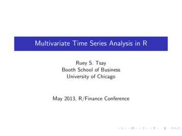
0.60.0ACFSeries resi[, 5]05101520252025Lag0.60.0ACFSeries resi[, 5] 2051015LagFigure: Autocorrelations of residuals and squared residuals of CanadianDollars

0.04 0.020.00x0.020.04Series with 2 Conditional SD Superimposed0100200300400500600IndexFigure: Volatility plot of log returns of Canadian Dollars

Summary 700.84541.3008Q(10, t )5.68(.8) 2.80(1.) 7.84(.6) 9.58(.5)Q(10, 2t .2019Q(10, t )4.46(.9) 5.86(.8) 11.42(.3)Q(10, 2t )235.341.4693.04

Motivation (continued)IIs there common volatility? (Global integration?Interdependence?)Although each series displays ARCH effects, is it possible to findsome linear combinations of these seven variables that mitigate theARCH effect? (to reduce risk)IIf yes, how to construct no-ARCH effect portfolios from theseseven exchange rates?

ARCH DimensionFor k assets, how to quantify volatility factors?Answer: ARCH dimension.Suppose yt (yi,t , · · · , yk,t )0 is a k-dimensional series withconditional mean zero, and a time-varying conditional covarianceΣt E (yt y0t Ωt 1 ),where Ωt 1 is the σ-field generated by {yt 1 , yt 2 , · · · }.

ARCH Dimension and TransformationISeek simplifying structure in Σt .ISuppose a k k matrix M (M01 , M02 )0 exists such that thetransformed series Myt [(M1 yt )0 , (M2 yt )0 ]0 satisfies C1 C2tE [Myt (Myt )0 Ωt 1 ] MΣt M0 ,C02t twhere t is an r r time-varying conditional covariance of M2 yt ,where 0 r k.

ARCH Dimension and TransformationIThe ARCH dimension of yt is r if a (k r ) k matrix M1 existssuch that Cov(M1 yt Ωt 1 ) M1 Σt M01 is a constant matrix.IThe M1 is referred to as a no-ARCH transformation.IEngle and Kozicki (1993) and Engle and Susmel (1993) discussed apairwise method to identify the common feature in volatility.

Generalized covariance matrixStatistics of interest:Volatility models are essentially concerned with the linear dynamicdependence of the matrix process {yt y0t t 1, . . . , T }.A multivariate ARCH(1) model:E (yt y0t Ωt 1 ) A0 A00 A1 (yt 1 y0t 1 )A01 .That is, elements of yt y0t relate to yi,t 1 yj,t 1 .

Generalized covariance matrix (cont.)IDefine the Generalized CovarianceCov(yt y0t , xt 1 ) [Cov(yit yjt , xt 1 )]where xt 1 Ωt 1 is a univariate random variable.IThe generalized covariance satisfies thatCov{Myt (Myt )0 , xt 1 } MCov(yt y0t , xt 1 )M0 .The idea has been used before, e.g. Li (1992, pHd method)

Generalized lag- cross-kurtosis matrixγ k XkXi 1 j iCov2 (yt y0t , yi,t yj,t ) k XkXγ 2 ,iji 1 j iwhereγ ,ij Cov(yt y0t , yi,t yj,t ),and the square is used to ensure non-negative definite of γ .Both γ ,ij and γ are k k symmetric matrix.

Implication of a zero eigenvalueConsider γ with fixed. Let u be a k-dimensional vectorassociated with a zero eigenvalue if it exists. That is, γ u 0.Then, γ 2 ,ij u 0, implyingγ ,ij u 0,for all i and j. This implies that yt y0t is not correlated withyi,t yj,t for all i, j.

Data Analysis: FXIRecall the data of seven exchange rates (k 7). Each returnseries contains 605 observations. A VAR(5) model is adoptedto remove the serial correlation to have residual series yt .IEach residual series displays ARCH effects. We ask ”whetherthere exists no-ARCH portfolios?”

Data Analysis (continue)Ibm for m 10 to estimate the transformation M,bWe adopt ΓPPP2kkm2cbm (yt y0t , yi,t h yj,t h ).where Γj i (1 h/n) covi 1h 1Ib .The estimates of principal volatility component are Myt