Transcription
Chapter 13Multivariate TechniquesChapter Table of ContentsIntroduction . . . . . . . . . . . . . . . . . . . . . . . . . . 279Principal Components Analysis . . . . . . . . . . . . . . . . 280Canonical Correlation . . . . . . . . . . . . . . . . . . . . . 289References . . . . . . . . . . . . . . . . . . . . . . . . . . . . 298
278 Chapter 13. Multivariate TechniquesSAS OnlineDoc : Version 8
Chapter 13Multivariate TechniquesIntroductionMultivariate analysis techniques, such as principal components analysis and canonical correlation, enable you to investigate relationshipsin your data. Unlike statistical modeling, you do this without designating dependent or independent variables. In principal componentanalysis, you examine relationships within a single set of variables.In canonical correlation analysis, you examine the relationship between two sets of variables.Figure 13.1.Multivariate MenuThe Analyst Application enables you to perform principal components analysis and canonical correlation. The Principal Componentstask enables you to compute principal components from a single setof variables. The Canonical Correlation task enables you to examinethe relationship between two sets of variables.The examples in this chapter demonstrate how you can use the Analyst Application to perform principal components and canonical correlation analyses.
280 Chapter 13. Multivariate TechniquesPrincipal Components AnalysisThe purpose of principal component analysis is to derive a smallnumber of independent linear combinations (principal components)of a set of variables that retain as much of the information in theoriginal variables as possible.For example, suppose you are interested in examining the relationship among measures of food consumption from different sources.The sample data set Protein records the amount of protein consumedfrom nine food groups for each of 25 European countries. The ninefood groups are red meat (RedMt), white meat (WhiteMt), eggs(Eggs), milk (Milk), fish (Fish), cereal (Cereal), starch (Starch),nuts (Nuts), and fruits and vegetables (FruVeg).Open the Protein Data SetThe data are provided in the Analyst Sample Library. To access thisAnalyst sample data set, follow these steps:1. Select Tools! Sample Data : : :2. Select Protein.3. Click OK to create the sample data set in your Sasuser directory.4. Select File! Open By SAS Name : : :5. Select Sasuser from the list of Libraries.6. Select Protein from the list of members.7. Click OK to bring the Protein data set into the data table.SAS OnlineDoc : Version 8
Principal Components Analysis 281Request the Principal Components AnalysisTo perform a principal components analysis, follow these steps:1. Select Statistics! Multivariate ! Principal Components : : :2. Highlight all of the quantitative variables (RedMt, WhiteMt,Eggs, Milk, Fish, Cereal, Starch, Nuts, and FruVeg).3. Click on the Variables button.The goal of this analysis is to determine the principal componentsof all protein sources. Therefore, all of the protein source variablesare included in the Variables list, as displayed in Figure 13.2. Thecharacter variable Country is an identifier variable and is omittedfrom the Variables list.Note that you can analyze a partial correlation or covariance matrixby specifying the variables to be partialed out in the Partial list. Thefull correlation matrix is used for this analysis.Figure 13.2.Principal Components DialogSAS OnlineDoc : Version 8
282 Chapter 13. Multivariate TechniquesThe default principal components analysis includes simple statistics,the correlation matrix for the analysis variables, and the associatedeigenvalues and eigenvectors.Request Principal Component PlotsYou can use the Plots dialog to request a scree plot or componentplots. A scree plot is useful in determining the appropriate numberof components to interpret. It displays the eigenvalues on the verticalaxis and the principal component number on the horizontal axis.To request a scree plot, follow these steps:1. Click on the Plots button in the main dialog.2. Select Create scree plot.Figure 13.3 displays the Scree Plot tab, in which a scree plot of thepositive eigenvalues is requested.Figure 13.3.SAS OnlineDoc : Version 8Principal Components: Plots Dialog, Scree Plot Tab
Principal Components Analysis 283A component plot displays the component score of each observationfor a pair of components. When you specify an Id variable, the valuesof that variable are also displayed in the plot.To request a component plot in addition to the scree plot, followthese steps.1. Click on the Component Plot tab in the Plots dialog.2. Select Create component plots.3. Click on the down arrow in the box labeled Type:4. Select Enhanced. An enhanced component plot displays thevariable names and values of the Id variable in the plot.5. Select the variable Country in the Id variable list.6. Click on the Id button to select the variable Country as an Idvariable.You can also enter the Dimensions for which you want plots. Forexample, to request plots of the first versus second, first versus third,and second versus third principal components, you type the values 1and 3.7. Click OK.Figure 13.4 displays the Component Plot tab, which requests anenhanced component plot.SAS OnlineDoc : Version 8
284 Chapter 13. Multivariate TechniquesFigure 13.4.Principal Components: Plots Dialog, ComponentPlot TabClick OK in the Principal Components dialog to perform the analysis.Review the ResultsFigure 13.5 displays simple statistics and correlations among thevariables.SAS OnlineDoc : Version 8
Principal Components AnalysisFigure 13.5. 285Principal Components: Simple Statistics and CorrelationsFigure 13.6 displays the eigenvalues and eigenvectors of the correlation matrix for the nine variables. The eigenvalues indicate that fourcomponents provide a reasonable summary of the data, accountingfor about 84% of the total variance. Subsequent components eachcontribute 5% or less.SAS OnlineDoc : Version 8
286 Chapter 13. Multivariate TechniquesFigure 13.6.Principal Components: Eigenvectors and EigenvaluesThe table of eigenvectors in Figure 13.6 reveals that the first eigenvector has equally large loadings on all of the animal-protein variables. This suggests that the first component is primarily a measureof animal-protein consumption. This eigenvector also has a largeloading on the variable Starch and negative loadings on the variables Cereal and Nuts.The second eigenvector has high positive loadings on the variablesFish, Starch, and FruVeg. This component seems to account fordiets in coastal regions or warmer climates. The remaining components are not as easily identified.The scree plot displayed in Figure 13.7 shows a gradual decreasein eigenvalues. However, the contributions are relatively low afterthe fourth component, which agrees with the preceding conclusionthat four principal components provide a reasonable summary of thedata.SAS OnlineDoc : Version 8
Principal Components AnalysisFigure 13.7. 287Principal Components: Scree PlotThe following enhanced component plot (Figure 13.8) displays therelationship between the first two components; each observation isidentified by country.SAS OnlineDoc : Version 8
288 Chapter 13. Multivariate TechniquesIn addition, the plot is enhanced to depict the correlations betweenthe variables and the components. This correlation is often called thecomponent loading. The amount by which each variable “loads” ona component is measured by its correlation with the component.Figure 13.8.SAS OnlineDoc : Version 8Principal Components:Loading PlotScores and Component
Canonical Correlation 289In Figure 13.8, each vector corresponds to one of the analysis variables and is proportional to its component loading. For example, thevariables Eggs, Milk, and RedMt all load heavily on the first component. The variables Fish and FruVeg load heavily on the secondcomponent but load very little on the first component.The information provided by the variable Country reveals that western European countries tend to consume protein from more expensive sources (that is, meat, eggs, and milk), while countries near theMediterranean Sea rely more heavily on fruits, vegetables, nuts, andfish for their protein sources. Eastern European countries rely moreon cereal crops and nuts to supply their protein.Canonical CorrelationCanonical correlation analysis is a variation on the concept of multiple regression and correlation analysis. In multiple regression andcorrelation analysis, you examine the relationship between a singleY variable and a linear combination of a set of X variables. In canonical correlation analysis, you examine the relationship between a linear combination of the set of Y variables and a linear combination ofthe set of X variables.For example, suppose that you want to determine the degree of correspondence between a set of job characteristics and measures ofemployee satisfaction. The sample data set Jobs contains the taskcharacteristics and satisfaction profiles for 14 jobs. The three variables associated with job satisfaction are career track satisfaction(Career), management and supervisor satisfaction (Supervis), andfinancial satisfaction (Finance). The three variables associated withjob characteristics are task variety (Variety), supervisor feedback(Feedback), and autonomy (Autonomy).In this task, the canonical correlation analysis is performed, labelsare specified to identify each set of canonical variables, and a plot ofthe canonical variables is requested.SAS OnlineDoc : Version 8
290 Chapter 13. Multivariate TechniquesOpen the Jobs Data SetThe data are provided in the Analyst Sample Library. To access thisAnalyst sample data set, follow these steps:1. Select Tools! Sample Data : : :2. Select Jobs.3. Click OK to create the sample data set in your Sasuser directory.4. Select File! Open By SAS Name : : :5. Select Sasuser from the list of Libraries.6. Select Jobs from the list of members.7. Click OK to bring the Jobs data set into the data table.Request the Canonical Correlation AnalysisTo perform a canonical correlation analysis, follow these steps:!Multivariate ! Canonical Correlation: : :1. Select Statistics2. Select the job satisfaction variables (Career, Supervis, andFinance) as the variables in Set 1.3. Select the job characteristic variables (Variety, Feedback,and Autonomy) as the variables in Set 2.Figure 13.9 displays the Canonical Correlation dialog, with each ofthe two sets of variables defined.SAS OnlineDoc : Version 8
Canonical CorrelationFigure 13.9. 291Canonical Correlation DialogThe default analysis includes the canonical correlations, eigenvalues,likelihood ratios, and tests of significance.Specify Identifying LabelsYou can optionally specify labels and prefixes to identify the twogroups of calculated canonical variables. To specify labels and prefixes, follow these steps:1. Click on the Statistics button in the main dialog.2. Enter a label for each of the two sets of canonical variables.3. Enter a prefix for each set of canonical variables. The prefix isused to assign names to the canonical variables.4. Click OK.Figure 13.10 displays the Canonical Analysis tab with labels andprefixes specified.SAS OnlineDoc : Version 8
292 Chapter 13. Multivariate TechniquesFigure 13.10.Canonical Correlation: Statistics Dialog, CanonicalAnalysis TabRequest Canonical Variate PlotsTo request plots of the canonical variables, follow these steps:1. Click on the Plots button in the main dialog.2. Select Create canonical variable plots.You can also enter the Canonical variables for which you wantplots. For example, to request plots of the first, second, and thirdcanonical variable pairs, you would type the values 1 and 3.3. Click OK.Figure 13.11 displays the Plots dialog, in which plots of the first twocanonical variables are requested.SAS OnlineDoc : Version 8
Canonical CorrelationFigure 13.11. 293Canonical Correlation: Plots DialogClick OK in the Canonical Correlation dialog to perform the analysis.Review the ResultsFigure 13.12 displays the canonical correlation, adjusted canonicalcorrelation, approximate standard error, and squared canonical correlation for each pair of canonical variables.Figure 13.12.Canonical Correlation: Correlations and EigenvaluesSAS OnlineDoc : Version 8
294 Chapter 13. Multivariate TechniquesThe first canonical correlation (the correlation between the first pairof canonical variables) is 0:9194. This value represents the highest possible correlation between any linear combination of the jobsatisfaction variables and any linear combination of the job characteristics variables.Figure 13.12 also displays the likelihood ratios and associated statistics for testing the hypothesis that the canonical correlations in thecurrent row and all that follow are zero. The first approximate Fvalue of 2:93 corresponds to the test that all three canonical correlations are zero. Since the p-value is small (0:0223), you can rejectthe null hypothesis at the 0:05 level. The second approximate F value of 0:49 corresponds to the test that both the second andthe third canonical correlations are zero. Since the p-value is large(0:7450), you fail to reject the hypothesis and conclude that only thefirst canonical correlation is significant at the 0:05 level.Several multivariate statistics and F test approximations are also provided. These statistics test the null hypothesis that all canonical correlations are zero. The small p-values for these tests ( 0:05), except for Pillai’s Trace, suggest rejecting the null hypothesis that allcanonical correlations are zero.SAS OnlineDoc : Version 8
Canonical CorrelationFigure 13.13. 295Canonical Correlation: Correlation CoefficientsEven though canonical variables are artificial, they can often be identified in terms of the original variables. To identify the variables,inspect the standardized coefficients of the canonical variables andthe correlations between the canonical variables and their originalvariables. Based on the results displayed in Figure 13.12, only thefirst canonical correlation is significant. Thus, only the first pair ofcanonical variables (Satisfy1 and Characteristic1) need to be identified.The standardized canonical coefficients in Figure 13.13 show that thefirst canonical variable for the Job Satisfaction group is a weightedsum of the variables Supervis (0:7854) and Career (0:3028), withthe emphasis on Supervis. The coefficient for the variable Financeis near 0. Therefore, a person satisfied with his or her supervisor andwith a large degree of career satisfaction would score high on thecanonical variable Satisfaction1.SAS OnlineDoc : Version 8
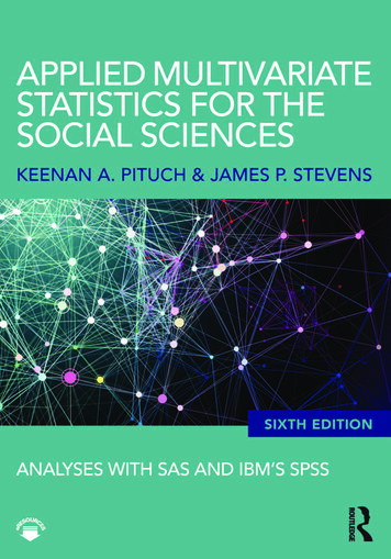
296 Chapter 13. Multivariate TechniquesThe coefficients for the Job Characteristics variables show that degree of autonomy (Autonomy) and amount of feedback (Feedback)contribute heavily to the Characteristic1 canonical variable (0:8403and 0:5520, respectively).Figure 13.14 displays the table of correlations between the canonical variables and the original variables. Although these univariatecorrelations must be interpreted with caution, since they do not indicate how the original variables contribute jointly to the canonicalanalysis, they are often useful in the identification of the canonicalvariables.Figure 13.14.SAS OnlineDoc : Version 8Canonical Correlation: Canonical Structure
Canonical Correlation 297As displayed in Figure 13.14, the supervisor satisfaction variable,Supervis, is strongly associated with the Satisfy1 canonical variable (r 0:9644). Slightly less influential is the variable Career,which has a correlation with the canonical variable of 0:7499. Thus,the canonical variable Satisfy1 seems to represent satisfaction withsupervisor and career track.The correlations for the job characteristics variables show that thecanonical variable Characteristic1 seems to represent all three measured variables, with the degree of autonomy variable (Autonomy)being the most influential (0:8459).Hence, you can interpret these results to mean that job characteristicsand job satisfaction are related. Jobs that possess a high degree ofautonomy and level of feedback are associated with workers who aremore satisfied with their supervisors and their careers. Additionally,the analysis suggests that, although the financial component is a factor in job satisfaction, it is not as important as the other satisfactionrelated variables.SAS OnlineDoc : Version 8
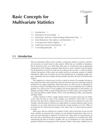
298 Chapter 13. Multivariate TechniquesFigure 13.15.Canonical Correlation: Plot of the First CanonicalVariablesThe plot of the first canonical variables, Satisfy1 and Characteristic1, is displayed in Figure 13.15. The plot depicts the strength ofthe relationship between the set of job satisfaction variables and theset of job characteristic variables.ReferencesSAS Institute Inc. (1999), SAS/STAT User’s Guide, Version 7-1,Cary, NC: SAS Institute Inc.SAS OnlineDoc : Version 8
The correct bibliographic citation for this manual is as follows: SAS Institute Inc.,The Analyst Application, First Edition, Cary, NC: SAS Institute Inc., 1999. 476 pp.The Analyst Application, First EditionCopyright 1999 SAS Institute Inc., Cary, NC, USA.ISBN 1–58025–446–2All rights reserved. Printed in the United States of America. No part of this publicationmay be reproduced, stored in a retrieval system, or transmitted, by any form or by anymeans, electronic, mechanical, photocopying, or otherwise, without the prior writtenpermission of the publisher, SAS Institute, Inc.U.S. Government Restricted Rights Notice. Use, duplication, or disclosure of thesoftware by the government is subject to restrictions as set forth in FAR 52.227–19Commercial Computer Software-Restricted Rights (June 1987).SAS Institute Inc., SAS Campus Drive, Cary, North Carolina 27513.1st printing, October 1999SAS and all other SAS Institute Inc. product or service names are registered trademarksor trademarks of SAS Institute Inc. in the USA and other countries. indicates USAregistration.IBM , ACF/VTAM , AIX , APPN , MVS/ESA , OS/2 , OS/390 , VM/ESA , and VTAM are registered trademarks or trademarks of International Business Machines Corporation. indicates USA registration.Other brand and product names are registered trademarks or trademarks of theirrespective companies.The Institute is a private company devoted to the support and further development of itssoftware and related services.
Multivariate analysis techniques, such as principal components anal-ysis and canonical correlation, enable you to investigate relationships in your data. Unlike statistical modeling, you do this without desig-nating dependent or independent variables. In principal component analysis, you examine relationships within a single set of variables.