WIXLIB

3-4 Ghil et al.: CLIMATIC TIME SERIES ANALYSIS40, 1 / REVIEWS OF GEOPHYSICSrelated from t to t 1, and Gaussian at each t, withconstant variance equal to unity. In the Yule [1927] andWalker [1931] method for the time domain approach,one computes the coefficients a j and the variance 2from a realization of X having length N, {X(t) 1 ⱕ t ⱕN }.[8] This method is discussed further in section 3.3below, where (1) is treated as an autoregressive (AR)process of order M, which we denote by AR(M). Thenotation used in the present paper is summarized inTable 1. The table lists the main symbols in alphabeticalorder and indicates the section where each symbol isintroduced first. This facilitates the comparison betweenthe methods we review, since the literature of eachmethod tends to use its own notation.[9] The spectral domain approach is motivated by theobservation that the most regular, and hence predictable, behavior of a time series is to be periodic. Thisapproach then proceeds to determine the periodic components embedded in the time series by computing theassociated periods, amplitudes, and phases, in this order.[10] The classical implementation of the spectral domain approach is based on the Bochner-Khinchin-Wiener theorem [Box and Jenkins, 1970], which states thatthe lag autocorrelation function of a time series and itsspectral density are Fourier transforms of each other.Hannan’s [1960] introduction to this approach and itsimplementation excels by its brevity and clarity; theso-called Blackman-Tukey implementation is presentedin section 3.2 below. We shall use here both the moremathematical term of spectral density and the term ofpower spectrum, often encountered in the scientific andengineering literature, according to whether the contextis more theoretical or more applied.[11] The remainder of this review is organized asfollows. Section 2 deals mainly with signal-to-noise (S/N)ratio enhancement and introduces singular spectrumanalysis (SSA) as an important and flexible tool for thisenhancement. Connections between SSA and empiricalorthogonal functions (EOFs) are outlined in AppendixA. Statistical tests for the reliability of SSA results arealso discussed in this section, along with connections towavelet analysis.[12] In section 3 we present, in succession, threemethods of spectral analysis: Fourier transform based,maximum entropy, and multitaper. Both sections 2 and 3use the SOI time series for the purposes of illustratingthe methods “in action.” In section 4 the multivariateextensions of the maximum entropy method and ofsingle-channel SSA are introduced, and a few additionalapplications are mentioned or illustrated. The reviewconcludes with a section on open questions, from thepoint of view of both the methodology and its applications.revolution” in time series analysis. Irregularity in observed time series had traditionally been attributed tothe above mentioned random “pumping” of a linearsystem by infinitely many (independent) degrees of freedom (DOF). In the 1960s and 1970s the scientific community found out that much of this irregularity could begenerated by the nonlinear interaction of a few DOF[Lorenz, 1963; Smale, 1967; Ruelle and Takens, 1971].This realization of the possibility of deterministic aperiodicity or “chaos” [Gleick, 1987] created quite a stir.[14] The purpose of this review is to describe brieflysome of the implications of this change in outlook fortime series analysis, with a special emphasis on climatictime series. Many general aspects of nonlinear timeseries analysis are reviewed by Drazin and King [1992],Ott et al. [1994], and Abarbanel [1996]. We concentratehere on those aspects that deal with regularities andhave proven most useful in studying climatic variability.[15] A connection between deterministically chaotictime series and the nonlinear dynamics generating themwas attempted fairly early in the young history of “chaostheory.” The basic idea was to consider specifically ascalar, or univariate, time series with apparently irregular behavior, generated by a deterministic or stochasticsystem. This time series could be exploited, so the thinking went, in order to ascertain, first, whether the underlying system has a finite number of DOF. An upperbound on this number would imply that the system isdeterministic, rather than stochastic, in nature. Next, wemight be able to verify that the observed irregularityarises from the fractal nature of the deterministic system’s invariant set, which would yield a fractional, ratherthan integer, value of this set’s dimension. Finally, onecould maybe reconstruct the invariant set or even theequations governing the dynamics from the data.[16] This ambitious program [Packard et al., 1980;Roux et al., 1980; Ruelle, 1981] relied essentially on themethod of delays, based in turn on the Whitney [1936]embedding lemma and the Mañé [1981] and Takens[1981] theorems. We first describe an easy connectionbetween a univariate and a multivariate time series.[17] Let us assume that the univariate time series isthe solution of a scalar nonlinear ODE of order p,1.2. Time Series and Nonlinear Dynamics[13] Before proceeding with the technical details, wegive in this section a quick perspective on the “nonlinearso that F 1 X 2 , F 2 X 3 , 䡠 䡠 䡠 , F p G. In other words,the successive derivatives of X(t) can be thought of asthe components of a vector X (X 1 , 䡠 䡠 䡠 , X p ). TheX 共 p兲 G共X 共 p 1兲, . . . , X兲.(2)This scalar higher-dimensional equation is equivalent tothe following system of first-order ODEs:Ẋ i F i共X 1, . . . , X j, . . . , X p兲,1 ⱕ i, j ⱕ p;(3)here Ẋ dX/dt X (1) and X ( p) d p X/dt p . It sufficesto writeX X 1, Ẋ 1 X 2, . . . , Ẋ p 1 X p, Ẋ p G共X 1, . . . , X p兲,(4)

40, 1 / REVIEWS OF GEOPHYSICSEuclidean space p in which the vector X X(t) evolvesis called the phase space of the first-order system (3).The graph of this evolution in p is called an orbit or atrajectory of equation (3).[18] Let us now change the point of view and considersystem (3) for arbitrary right-hand sides F i (X), ratherthan for the specific F i given by (4). Such an ODEsystem represents a fairly general description of a differentiable dynamical system in continuous time [Arnold, 1973, 1983]. We are interested at first in the case inwhich only a single time series X̂(t) is known, where X̂ X i for some fixed component i i 0 or X̂ is somesufficiently smooth function of all the components X i .For the solutions of such a system to be irregular, i.e.,other than (asymptotically) steady or periodic, three ormore DOF are necessary. Can one then go from (3) to(2) just as easily as in the opposite direction? Theanswer, in general is no; hence a slightly more sophisticated procedure needs to be applied.[19] This procedure is called the method of delays,and it tries, in some sense, to imitate the Yule-Walkerinference of (1) from the time series {X(t) t 1, 䡠 䡠 䡠 ,N }. First of all, one acknowledges that the data X(t) aretypically given at discrete times t n t only. Next, oneadmits that it is hard to actually get the right-hand sidesF i ; instead, one attempts to reconstruct the invariant seton which the solutions of (3) that satisfy certain constraints lie.[20] In the case of conservative, Hamiltonian systems[Lichtenberg and Lieberman, 1992], there are typicallyunique solutions through every point in phase space.The irregularity in the solutions’ behavior is associatedwith the intricate structure of cantori [Wiggins, 1988],complicated sets of folded tori characterized by a givenenergy of the solutions lying on them. These cantorihave, in particular, finite and fractional dimension, beingself-similar fractals [Mandelbrot, 1982].[21] Mathematically speaking, however, Hamiltoniansystems are structurally unstable [Smale, 1967] in thefunction space of all differentiable dynamical systems.Physically speaking, on the other hand, “open” systems,in which energy is gained externally and dissipated internally, abound in nature. Therefore climatic time series, as well as most other time series from nature or thelaboratory, are more likely to be generated by forceddissipative systems [Lorenz, 1963; Ghil and Childress,1987, chapter 5]. The invariant sets associated with irregularity here are “strange attractors” [Ruelle and Takens, 1971], toward which all solutions tend asymptotically; that is, long-term irregular behavior in suchsystems is associated with these attractors. These objectsare also fractal, although rigorous proofs to this effecthave been much harder to give than in the case ofHamiltonian cantori [Guckenheimer and Holmes, 1983;Lasota and Mackey, 1994].[22] Mañé [1981], Ruelle [1981], and Takens [1981]had the idea, developed further by Sauer et al. [1991],that a single observed time series X̂(t) (where X̂ X i 0Ghil et al.: CLIMATIC TIME SERIES ANALYSIS or, more generally, X̂ (X 1 (t), 䡠 䡠 䡠 , X p (t))) could beused to reconstruct the attractor of a forced dissipativesystem. The basis for this reconstruction idea is essentially the fact that the solution that generates X(t) coversthe attractor densely; that is, as time increases, thissolution will pass arbitrarily close to any point on theattractor. Time series observed in the natural environment, however, have finite length and sampling rate, aswell as significant measurement noise.[23] The embedding idea has been applied thereforemost successfully to time series generated numerically orby laboratory experiments in which sufficiently long series could be obtained and noise was controlled betterthan in nature. Broomhead and King [1986a], for instance, successfully applied SSA to the reconstruction ofthe Lorenz [1963] attractor. As we shall see, for climateand other geophysical time series, it might be possible toattain a more modest goal: to describe merely a “skeleton” of the attractor that is formed by a few robustperiodic orbits.[24] In the climate context, Lorenz [1969] had alreadypointed out a major stumbling block for applying theattractor reconstruction idea to large-scale atmosphericmotions. While using more classical statistical methods,he showed that the recurrence time of sufficiently goodanalogs for weather maps was of the order of hundredsof years, at the spatial resolution of the observationalnetwork then available for the Northern Hemisphere.[25] The next best target for demonstrating from anobserved time series the deterministic cause of its irregularity was to show that the presumed system’s attractorhad a finite and fractional dimension. Various dimensions, metric and topological, can be defined [Kaplanand Yorke, 1979; Farmer et al., 1983]; among them, theone that became the most popular, since easiest tocompute, was the correlation dimension [Grassbergerand Procaccia, 1983]. In several applications, its computation proved rather reliable and hence useful. Climatictime series, however, tended again to be rather too shortand noisy for comfort (see, for instance, Ruelle [1990]and Ghil et al. [1991] for a review of this controversialtopic).[26] A more robust connection between classical spectral analysis and nonlinear dynamics seems to be provided by the concept of “ghost limit cycles.” The road tochaos [Eckmann, 1981] proceeds from stable equilibria,or fixed points, through stable periodic solutions, or limitcycles, and on through quasiperiodic solutions lying ontori, to strange attractors. The fixed points and limitcycles are road posts on this highway from the simple tothe complex. That is, even after having lost their stabilityto successively more complex and realistic solutions,these simple attractors still play a role in the observedspatial patterns and the time series generated by thesystem.[27] A “ghost fixed point” is a fixed point that hasbecome unstable in one or a few directions in phasespace. Still, the system’s trajectories will linger near it for3-5

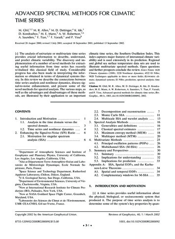
3-6 Ghil et al.: CLIMATIC TIME SERIES ANALYSIS40, 1 / REVIEWS OF GEOPHYSICSsection 2.2, how this concept can be generalized toassociate multiple spectral peaks with a robust skeletonof the attractor, as proposed by Vautard and Ghil [1989].Figure 1. Schematic diagram of a ghost limit cycle. Figure 1ais a perspective sketch of the limit cycle (bold curve) in athree-dimensional Euclidean space. Light solid curves indicatetwo distinct trajectories that approach the limit cycle in adirection in which it is stable and leave its neighborhood in anunstable direction. Figure 1b is a sketch of the projection offour representative trajectories (light curves) onto a Poincarésection (i.e., a plane intersecting transversally the limit cycle) ina neighborhood of the limit cycle. The figure’s mutually perpendicular directions (bold lines) of stability (inward pointingarrows) and instability (outward pointing arrows) can form, ingeneral, an arbitrary angle with each other. The shape of sucha limit cycle need not be elliptic, as shown in the figure, exceptnear the Hopf bifurcation point where it arises. Reprintedfrom Ghil and Yiou [1996] with permission of Springer-Verlag.extended time intervals [Legras and Ghil, 1985]. Likewise, a ghost limit cycle is a closed orbit that has becomeslightly unstable but is visited, again and again, by thesystem’s trajectories [Kimoto and Ghil, 1993].[28] Consider the periodic solution shown in Figure1a as embedded in Euclidean three-dimensional phasespace. It is neutrally stable in the direction tangent toitself, while in the plane perpendicular to this tangent itis asymptotically stable in one direction and unstable inthe other, as shown in the Poincaré section of Figure 1b.In a multidimensional phase space it is plausible that thedirections of stability are numerous or even infinite innumber. The directions of instability, however, wouldstill be few in number, for parameter values not too farfrom those at which the Hopf bifurcation that gave riseto the limit cycle in the first place occurs. Hence solutions of the full system would easily be attracted to thisbarely unstable limit cycle, follow it closely for one or afew turns, be ejected from its neighborhood, only toreturn later, again and again.[29] The analogous picture for a ghost fixed point wasillustrated in detail for an atmospheric model with 25DOF by Legras and Ghil [1985; see also Ghil and Childress, 1987, Figures 6.12 and 6.18]. Thus the “ghosts” offixed points and limit cycles leave their imprint on thesystem’s observed spatiotemporal behavior.[30] The episodes during which the system trajectorycircles near a ghost limit cycle result in nearly periodicsegments of the time series and hence contribute to aspectral peak with that period. This concept was illustrated using 40 years of an atmospheric multivariate timeseries by Kimoto and Ghil [1993] for the so-called intraseasonal oscillations of the Northern Hemisphere[see also Ghil and Mo, 1991a]. We shall show in thesubsequent sections of the present review, in particular2. ENHANCING THE SIGNAL-TO-NOISE(S/N) RATIO2.1. Motivation for Singular Spectrum Analysis (SSA)[31] SSA is designed to extract information from shortand noisy time series and thus provide insight into theunknown or only partially known dynamics of the underlying system that generated the series [Broomheadand King, 1986a; Fraedrich, 1986; Vautard and Ghil,1989]. We outline here the method for univariate timeseries and generalize for multivariate ones in section 4.2.[32] The analogies between SSA and spatial EOFs aresummarized in Appendix A, along with the basis of bothin the Karhunen-Loève theory of random fields and ofstationary random processes. Multichannel SSA (seesection 4.2) is numerically analogous to the extendedEOF (EEOF) algorithm of Weare and Nasstrom [1982].The two different names arise from the origin of theformer in the dynamical systems analysis of univariatetime series, while the latter had its origins in the principal component analysis of meteorological fields. The twoapproaches lead to different methods for the choice ofkey parameters, such as the fixed or variable windowwidth, and hence to differences in the way of interpreting results.[33] The starting point of SSA is to embed a timeseries {X(t) t 1, 䡠 䡠 䡠 , N } in a vector space of dimension M, i.e., to represent it as a trajectory in the phasespace of the hypothetical system that generated {X(t)}.In concrete terms this is equivalent to representing thebehavior of the system by a succession of overlapping“views” of the series through a sliding M-point window.[34] Let us assume, for the moment, that X(t) is anobservable function X̂(t) of a noise-free system’s dependent variables X i (t), as defined in (4), and that thefunction that maps the p variables {X i (t) i 1, 䡠 䡠 䡠 ,p} into the single variable X(t) has certain propertiesthat make it generic in the dynamical systems sense ofSmale [1967]. Assume, moreover, that M 2d 1,where d is the dimension of the underlying attractor onwhich the system evolves, and that d is known and finite.If so, then the representation of the system in the “delaycoordinates” described in (5) below will share key topological properties with a representation in any coordinate system. This is a consequence of Whitney’s [1936]embedding lemma and indicates the potential value ofSSA in the qualitative analysis of the dynamics of nonlinear systems [Broomhead and King, 1986a, 1986b;Sauer et al., 1991]. The quantitative interpretation ofSSA results in terms of attractor dimensions is fraughtwith difficulties, however, as pointed out by a number ofauthors [Broomhead et al., 1987; Vautard and Ghil, 1989;Palus̆ and Dvor̆ák, 1992].

40, 1 / REVIEWS OF GEOPHYSICSGhil et al.: CLIMATIC TIME SERIES ANALYSIS [35] We therefore use SSA here mainly (1) for dataadaptive signal-to-noise (S/N) enhancement and associated data compression and (2) to find the attractor’sskeleton, given by its least unstable limit cycles (seeagain Figure 1 above). The embedding procedure applied to do so constructs a sequence {X̃(t)} of Mdimensional vectors from the original time series X, byusing lagged copies of the scalar data {X(t) 1 ⱕ t ⱕN },X̃共t兲 共X共t兲, X共t 1兲, . . . , X共t M 1兲兲;(5)the vectors X̃(t) are indexed by t 1, 䡠 䡠 䡠 , N , where N N M 1.[36] SSA allows one to unravel the information embedded in the delay-coordinate phase space by decomposing the sequence of augmented vectors thus obtainedinto elementary patterns of behavior. It does so byproviding data-adaptive filters that help separate thetime series into components that are statistically independent, at zero lag, in the augmented vector space ofinterest. These components can be classified essentiallyinto trends, oscillatory patterns, and noise. As we shallsee, it is an important feature of SSA that the trendsneed not be linear and that the oscillations can beamplitude and phase modulated.[37] SSA has been applied extensively to the study ofclimate variability, as well as to other areas in the physical and life sciences. The climatic applica

time. Thus the SOI time series, as well as most climatic and other geophysical time series, are available in dis-crete time. 1.1. Analysis in the Time Domain Versus the Spectral Domain [5] Two basic approaches to time series analysis are associated with the time domain or the spectral domai