WIXLIB

An Introduction toSOLIDWORKS FlowSimulation 2017 John E. Matsson, Ph.D.SDCP U B L I C AT I O N SBetter Textbooks. Lower Prices.www.SDCpublications.com

Visit the following websites to learn more about this book:Powered by TCPDF (www.tcpdf.org)

Flat Plate Boundary LayerChapter 2Flat Plate Boundary LayerObjectives Creating the SOLIDWORKS part needed for the Flow SimulationSetting up Flow Simulation projects for internal flowSetting up a two-dimensional flow conditionInitializing the meshSelecting boundary conditionsInserting global goals, point goals and equation goals for the calculationsRunning the calculationsUsing Cut Plots to visualize the resulting flow fieldUse of XY Plots for velocity profiles, boundary layer thickness, displacement thickness,momentum thickness and friction coefficientsUse of Excel templates for XY PlotsComparison of Flow Simulation results with theories and empirical dataCloning of the projectProblem DescriptionIn this chapter, we will use SOLIDWORKS Flow Simulation to study the two-dimensionallaminar and turbulent flow on a flat plate and compare with the theoretical Blasius boundary layersolution and empirical results. The inlet velocity for the 1 m long plate is 5 m/s and we will beusing air as the fluid for laminar calculations and water to get a higher Reynolds number forturbulent boundary layer calculations. We will determine the velocity profiles and plot theprofiles using the well-known boundary layer similarity coordinate. The variation of boundarylayer thickness, displacement thickness, momentum thickness and the local friction coefficientwill also be determined. We will start by creating the part needed for this simulation; see figure2.0.Figure 2.0 SOLIDWORKS model for flat plate boundary layer studyChapter 2 - 1 -

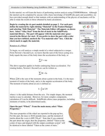
Flat Plate Boundary LayerCreating the SOLIDWORKS Part1. Start by creating a new part in SOLIDWORKS: select File New and click on the OK button inthe New SOLIDWORKS Document window. Click on Front Plane in the FeatureManagerdesign tree and select Front from the View Orientation drop down menu in the graphicswindow.Figure 2.1a) Selection of front planeFigure 2.1b) Selection of front view2. Click on the Sketch tab and select Corner Rectangle.Figure 2.2 Selecting a sketch tool3. Make sure that you have MMGS (millimeter, gram, second) chosen as your unit system. You cancheck this by selecting Tools Options from the SOLIDWORKS menu and selecting theDocument Properties tab followed by clicking on Units. Check the circle for MMGS and clickon the OK button to close the window. Click to the left and below the origin in the graphicswindow and drag the rectangle to the right and upward. Fill in the parameters for the rectangle:1000 mm wide and 100 mm high; see Figure 2.3b). Close the Rectangle dialog box by clicking on. Right click in the graphics window and select Zoom/Pan/Rotate Chapter 2 - 2 -Zoom to Fit.

Flat Plate Boundary LayerFigure 2.3a) Parameter settings for the rectangleFigure 2.3b) Zooming in the graphics window4. Repeat steps 2 and 3 but create a larger rectangle outside of the first rectangle. Dimensions areshown in figure 2.4.Figure 2.4 Dimensions of second larger rectangleChapter 2 - 3 -

Flat Plate Boundary Layer5. Select Features tab and Extruded Boss/Base. Check the box forOK to exit the Boss-Extrude Property Manager.Direction 2 and clickFigure 2.5a) Selection of extrusion featureFigure 2.5b) Closing the property manager6. Select Front from the View Orientation drop down menu in the graphics window. Click onFront Plane in the FeatureManager design tree. Click on the Sketch tab and select the Linesketch tool.Figure 2.6 Selection of the line sketch toolChapter 2 - 4 -

Flat Plate Boundary Layer7. Draw a vertical line in the Y-direction in the front plane starting at the lower inner surface of thesketch. Set the Parameters and Additional Parameters to the values shown in figure 2.7. Closethe Line Properties dialogand the Inert Line dialog.Figure 2.7 Parameters for vertical line8. Repeat steps 6 and 7 three more times and add three more vertical lines to the sketch: the secondline at X 400 mm with a length of 40 mm, the third line at X 600 mm with a length of 60 mmand the fourth line at X 800 mm with a length of 80 mm. These lines will be used to plot theboundary layer velocity profiles at different streamwise positions along the flat plate. Close theLine Properties dialogand the Insert Line dialog. Save the SOLIDWORKS part with thefollowing name: Flat Plate Boundary Layer Study 2017. Rename the newly created sketch inthe FeatureManager design tree; see figure 2.8. You will need to left click twice to rename thesketch.Figure 2.8 Renaming the sketch for boundary layer velocity profilesChapter 2 - 5 -

Flat Plate Boundary Layer9. Click on the Rebuild symbolin the SOLIDWORKS menu. Repeat step 6 and draw ahorizontal line in the X-direction starting at the origin of the lower inner surface of the sketch. Setthe Parameters and Additional Parameters to the values shown in figure 2.9 and close the LineProperties dialog and the Insert Line dialog. Rename the sketch in the FeatureManager designtree and call it x 0 – 0.9 m. Click on the Rebuild symbol.Figure 2.9 Sketching a line in the X-direction10. Next, we will create a split line. Repeat step 6 once again but this time select the Top Plane anddraw a line in the Z-direction through the origin of the lower inner surface of the sketch. It willhelp to zoom in and rotate the view to complete this step. Set the Parameters and AdditionalParameters to the values shown in figure 2.10 and close the dialog. Click on the Rebuildsymbol.Figure 2.10 Drawing a line in the Z-directionChapter 2 - 6 -

Flat Plate Boundary Layer11. Rename the new sketch in the FeatureManager design tree and call it Split Line. SelectInsert Curve Split Line from the SOLIDWORKS menu. Select Projection under Typeto Split. Select Split Line for Sketch to Project under Selections. For Faces to Split, select thesurface where you have drawn your split line; see figure 2.11b). Close the dialognow finished the part for the flat plate boundary layer. Select File Save from theSOLIDWORKS menu.Figure 2.11a) Creating a split lineFigure 2.11b) Selection of surface for the split lineChapter 2 - 7 -. You have

Flat Plate Boundary LayerSetting Up the Flow Simulation Project12. If Flow Simulation is not available in the menu, you have to add it from SOLIDWORKS menu:Tools Add Ins and check the corresponding SOLIDWORKS Flow Simulation 2017 boxunder SOLIDWORKS Add-Ins and click OK to close the Add-Ins window. Select Tools FlowSimulation Project Wizard to create a new Flow Simulation project. Enter Project name:“Flat Plate Boundary Layer Study.” Click on the Next button. Select the default SI (m-kg-s)unit system and click on the Next button once again.Figure 2.12a) Starting a new Flow Simulation projectFigure 2.12b) Creating a name for the project13. Use the default Internal Analysis type and click on the Next button once again.Figure 2.13 Excluding cavities without flow conditionsChapter 2 - 8 -

Flat Plate Boundary Layer14. Select Air from the Gases and add it as Project Fluid. Select Laminar Only from the FlowType drop down menu. Click on the Next button. Use the default Wall Conditions and clickon the Next button. Insert 5 m/s for Velocity in X direction as Initial Conditions and click onthe Finish button. You will get a fluid volume recognition failure message. Answer Yes to thisquestion and create a lid on each side of the model. Answer Yes to the questions when you createthe lids.Figure 2.14 Selection of fluid for the project and flow type15. Select Tools Flow Simulation Computational Domain . Click on the 2D simulationbutton under Type and select XY plane. Close the Computational Domain dialogFigure 2.15a) Modifying the computational domainFigure 2.15b) Selecting 2D simulation in the XY planeChapter 2 - 9 -.

Flat Plate Boundary Layer16. Select Tools Flow Simulation Global Mesh . Select Manual under Type. Change NX to300 and NY to 200. Click on the OK button (green check mark) to exit the Initial Mesh window.Figure 2.16a) Modifying the initial meshFigure 2.16b) Changing the number of cells in two directionsSelecting Boundary Conditions17. Select theFlow Simulation analysis tree tab, open the Input Data folder by clicking onthe plus sign next to it and right click on Boundary Conditions. Select Insert BoundaryCondition . Select Wireframe as the Display Style. Right click in the graphics window andselect Zoom/Pan/Rotate Zoom to Fit. Once again, right click in the graphics window andselect Zoom/Pan/Rotate Rotate View. Click and drag the mouse so that the inner surface ofthe left boundary is visible. Right click again and unselect Zoom/Pan/Rotate Rotate View.Right click on the left inflow boundary surface and select Select Other. Select the Facecorresponding to the inflow boundary. Select Inlet Velocity in the Type portion of the BoundaryCondition window and set the velocity to 5 m/s in the Flow Parameters window. Click OK toexit the window. Right click in the graphics window and selectarea around the left boundary.Chapter 2 - 10 -Zoom to Area and select an

Flat Plate Boundary LayerFigure 2.17a) Inserting boundary conditionFigure 2.17b) Modifying the viewFigure 2.17c) Velocity boundary condition on the inflowChapter 2 - 11 -

Flat Plate Boundary LayerFigure 2.17d) Inlet velocity boundary condition indicated by arrows18. Red arrows pointing in the flow direction appear indicating the inlet velocity boundary condition;see figure 2.17d). Right click in the graphics window and select Zoom to Fit. Right click again inthe graphics window and selectRotate View once again to rotate the part so that the innerright surface is visible in the graphics window. Right click and click onSelect. Right clickonBoundary Conditions in the Flow Simulation analysis tree and select InsertBoundary Condition . Right click on the outflow boundary surface and select Select Other.Select the Face corresponding to the outflow boundary. Click on the Pressure Openings buttonin the Type portion of the Boundary Condition window and select Static Pressure. Click OK toexit the window. If you zoom in on the outlet boundary you will see blue arrows indicating thestatic pressure boundary condition; see figure 2.18b).Figure 2.18a) Selection of static pressure as boundary condition at the outlet of the flow regionChapter 2 - 12 -

Flat Plate Boundary LayerFigure 2.18b) Outlet static pressure boundary condition19. Enter the following boundary conditions: Ideal Wall for the lower and upper walls at the inflowregion; see figures 2.19. These will be adiabatic and frictionless walls.Figure 2.19 Ideal wall boundary condition for two wall sectionsChapter 2 - 13 -