Transcription
Available online at www.sciencedirect.comScienceDirectProcedia CIRP 29 (2015) 656 – 661The 22nd CIRP conference on Life Cycle EngineeringNetwork Design and Optimization for Multi-product, Multi-time, Multiechelon Closed-loop Supply Chain under UncertaintyAnil Jindal*, Kuldip Singh Sangwan, and Sachin SaxenaDepartment of Mechanical Engineering, Birla Institute of Technology and Science, Pilani, Rajasthan – 333031, India* Corresponding author. Tel.: 91-1596-515-852; fax: 91-1596-244-183. E-mail address: aniljindal1981@gmail.com, aniljindal@pilani.bits-pilani.ac.inAbstractThis paper proposes the network design and optimization of a multi-product, multi-time, multi-echelon capacitated closed-loop supply chain inan uncertain environment. The uncertainty related to ill-known parameters like product demand, return volume, fraction of parts recovered fordifferent product recovery processes, purchasing cost, transportation cost, inventory cost, processing, and set-up cost at facility centers ishandled with fuzzy numbers. A fuzzy mixed-integer linear programming model is proposed to decide optimally the location and allocation ofproducts/parts at each facility, number of products to be remanufactured, number of parts to be purchased from external suppliers and inventorylevel of products/parts in order to maximize the profit to the organization. The proposed solution methodology is able to generate a balancedsolution between the feasibility degree and the degree of satisfaction of the decision maker. The proposed model has been tested with anillustrative example. 20152015 TheThe Authors.Authors. PublishedPublished byby ElsevierElsevier B.V.B.V. This is an open access article under the CC BY-NC-ND licensePeer-reviewunder responsibility of the International Scientific Committee of the Conference “22nd CIRP conference on Life /4.0/).Engineering.Peer-review under responsibility of the scientific committee of The 22nd CIRP conference on Life Cycle EngineeringKeywords: Closed-loop supply chain; Product recovery; Fuzzy MILP; Reverse Logistics1. IntroductionClosed-loop supply chain (CLSC) is an environmentallyand economically sound way to achieve many of the goals ofsustainable development [1]. It has many benefits over thetraditional supply chain [2], but it also complicates themanagement and control of traditional supply chain [3]. It isfurther complicated by the uncertainty in quantity, quality andtiming of the return [4-5]. This uncertainty affects thepercentage of products/parts recovered from different productrecovery options like reuse, refurbish, recycle, and disposal,which further affect the inventory level of products and partsas well as the processing and set-up cost at various facilitycentres. Therefore, in this uncertain environment, determiningthe number of products to be remanufactured; the number ofparts to be directly purchased; inventory level of product andparts; and the location and allocation of external supplier(s),collection centre(s), disassembly centre(s), refurbishingcentre(s), recycling centre(s), and disposal centre(s) ischallenging to maximize the profit to the organization.This paper proposes the network design and optimizationof a multi-product, multi-time and multi-echelon capacitatedCLSC in an uncertain environment. The uncertainty related toill-known parameters is handled with triangular fuzzynumbers. The proposed CLSC network is presented by afuzzy mixed-integer linear programming model to decideoptimally the location and allocation of parts at each facility,inventory level of parts, number of products to beremanufacturer, and number of parts to be purchased fromexternal suppliers in order to maximize the profit oforganization. The proposed framework is tested by solving anillustrative CLSC network problem using the methodologyproposed by Jiménez et al. [6]. The advantage of themethodology is that it allows working with the concept offeasibility degree to find an optimal solution between twoconflicting objectives, i.e. to improve the objective functionvalue and the degree of satisfaction of constraintssimultaneously.The paper is organized as follows. The next sectionpresents the literature review. The proposed CLSC framework2212-8271 2015 The Authors. Published by Elsevier B.V. This is an open access article under the CC BY-NC-ND nd/4.0/).Peer-review under responsibility of the scientific committee of The 22nd CIRP conference on Life Cycle Engineeringdoi:10.1016/j.procir.2015.01.024
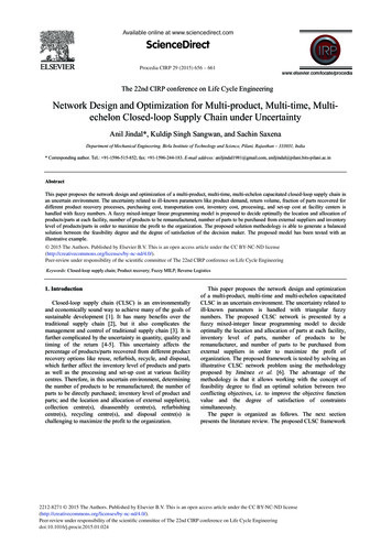
657Anil Jindal et al. / Procedia CIRP 29 (2015) 656 – 661is introduced in section 3 and the mathematical model for theproposed framework is given in section 4. The solutionmethodology is discussed in section 5 and section 6 is devotedto an illustrative example to test the model. Finally, in Section7 conclusions are presented.2. Literature reviewIn recent years there has been a growing awareness of theimportance of incorporating CLSC activities along with thetraditional indicators [7]. Lee and Dong [8] discussed thatreverse logistics network has a strong influence on theforward logistics and vice versa, therefore, the design of theforward and reverse logistics network should be integrated.Various strategic and operational aspects of CLSC havebeen investigated in the last decade. Beamon and Fernandes[9] proposed a single product, multi-time capicated locationand allocation model. Kim et al. [10] developed a multiperiod, multi-product mixed integer programming model withcrisp parameters. However, in the framework onlyrefurbishment and disposal of parts is considered and therepair, reuse and recycle of products/parts is not considered.Kannan et al. [11] compared the results of genetic algorithmand particle swarm optimization for the design of multiproduct and multi-time CLSC model. Mutha and Pokharel[12] presented location-allocation model to optimize the costby considering the modular product structure with differentdisposal and recycling fractions for each module. However,the model assumed deterministic demands by historicalaverage. Özceylan and Paksoy [7] proposed a mixed-integermathematical model for the location of plant and retailers inCLSC network. Amin and Zhang [13] proposed a two phasemulti-objective model to maximize profit and weights ofsuppliers, and to minimize defect rates. Shi et al. [5] proposeda mathematical model based on Lagrangian relaxation methodto investigate a CLSC network in which demand and returnare uncertain. Özceylan and Paksoy [7] proposed a multiechelon, multi-time period MILP model to minimize the totalcost. The uncertainty in percentage of products recovered ishandled with scenario analysis. Özceylan and Paksoy [14]proposed a fuzzy multi-objective model to take into accountthe fuzziness in the capacity, objectives, demand constraints,and reverse rates.From the above literaure review it can be observed thatmost of the CLSC models are single time period models [1519] and a few are multi-time period models [7, 9-10, 12].Therefore, there is a need to develop a multi-product, multitime, multi-echelon capacitated CLSC framework andoptimization model including product acquisition cost,transportation cost, purchasing cost, inventory cost,processing and set-up costs simultaneously considering theuncertainty in ill-know parameters.3. Proposed closed loop supply chain frameworkA generalized CLSC framework is presented for handlingmulti-product, multi-time, multi-echelon returns in whichforward flow, reverse flow and their mutual interactions areconsidered simultaneously (Figure 1). The proposedframework is an extension of the previous work [20], which isa single time period model without considering the inventorylevel of products and parts and the related inventory costs.It is assumed that the remanufactured products have samequality as the brand-new products and can be sold with thesame price [9-10]. Secondly that only parts of products can bedisposed off or recycled and not the whole product [21]. Theobjective of the model is to maximize the profit to theorganization by optimally determining the number of parts tobe purchased from external supplier(s) and the number ofproducts to be remanufactured under capacity constraints;location and allocation to different facility centres andinventory level of parts to meet the product demand. D jt D jtPjtManufacturerDistributorCustomersRetailerK jExternalSuppliers (k)SiktPartInventoryJ AjmtjCjmtFiltRefurbishingCenters (l)Forward LogisticsReverse LogisticsFinlt OiRjmntDisassemblyCenters (n)Yint ERecycle CenteriI iCollection and RepairCenters (m) withProduct inventoryWintDisposal CenterFig. 1 The proposed closed loop supply chain framework4. The proposed fuzzy mixed-integer linear programmingmodel (Fuzzy MILP)The proposed Fuzzy MILP model represents the proposedframework in mathematical terms for optimization.Indicesjikmnltset of products, j 1, 2, .Jset of parts, i 1, 2, .Iset of suppliers, k 1, 2, .Kset of collection/repair centres, m 1, 2, .Mset of disassembly centres, n 1, 2, .Nset of refurbishing centres, l 1, 2, .Lset of time periods, t 1, 2, .TDecision variablesunits of product j to be produced at time tPjtunits of product j to be collected at collection centreCjmtm at time tunits of product j reused from collection centre m atAjmttime tunits of product j disassembled at site n fromRjmntcollection centre m at time t(PI)jmt inventory level of product j at collection centre m attime t(PrI)it inventory level of part i at time tunits of part i purchased from supplier k at time tSiktunits of part i obtained at disassembly site n at time tTintunits of parts i refurbished at site l from disassemblyFinltcentre n at time tunits of part i refurbished at refurbishing centre l atFilttime tunits of part i disposed from disassembly centre n atWinttime tunits of part i recycled from disassembly centre n atYinttime tbinary variable for set-up of collection facility forBjmt
658Anil Jindal et al. / Procedia CIRP 29 (2015) 656 – 661VjntUiltproduct j at m at time tbinary variable for set-up of disassembly site forproduct j at n at time tbinary variable for set-up of refurbishing site for parti at l at time tParameters demand of product j to be produced at time tD jt ( PF ) jprofit by selling the product jqijunits of part i in product j( MP) jt plant capacity to produce product j at time t (CC ) jm unit cost of collection and inspection for product j atcollection centre m ( SC ) jm set-up cost for collection of product j at centre m( MC) jmt capacity of collection centre m for product j at time t ( DC ) in unit cost of disassembly for part i at disassemblycentre n ( SD) jn set-up cost for disassembly of product j at centre nand reused products. Equation (3), (4) and (5) represents theflow balance constraint at collection centre, disassemblycentre and refurbishing centre respectively. While equation(6), (7) and (8) calculate the number of parts at disassemblycentres, number of parts at refurbishing centres and number ofproducts at disassembly centres respectively. Constraints (9),(10), (11), and (12) provide the maximum limit on the numberof products collected, number of products reused, number ofparts refurbished and number of parts to be recycledrespectively. Constraints (13), (14), (15) and (17) ensure thecapacity limit for collection centre, disassembly centre,refurbishing centre and plant respectively. Constraint (16)ensures the maximum and minimum capacity of the externalsuppliers. The constraints (18) and (19) are related to binaryand general integer values of the decision variables. All thedecision variables are positive numbers.Objective FunctionMaximize ( PF j ) * ( Pjt A jmt ) ( RP ) i * Yinttmjtni( MD) jnt capacity of disassembly centre n for product j at time ( PC ) ik * S ikt (CC ) jm * C jmtt ( RC ) il unit cost of refurbishing for part i at centre l ( SR ) il set-up cost for refurbishing of part i at centre l( MR) ilt capacity of refurbishing centre l for part i at time t (UC ) jm unit cost of repair for product j from collection centre ( SC ) jm * B jmt (UC ) jm * A jmtm unitcost of disposal for part i(WDC ) i ( RP ) i unit profit of recycling for part i ( RF ) jm unit cost of refund to customers for product j ( PC ) ik unit purchasing cost for part i from supplier k (Pr I C ) it unit inventory cost of part i at time t ( PI C ) jmt unit inventory cost of product j at collection centre mat time tmaximum and minimum purchase( MXS) k , (MNS) korder from supplier k (TCD) jmn unit cost of transportation from collection centre mto disassembly centre n for product j (TCR) inl unit cost of transportation from disassembly centre nto refurbishing centre l for part i (TCU ) jm unit cost of transportation from collection/repaircentre m to distributor for product jMaximum percentage of product j returnedK jMaximum percentage of product j reusedJ j Oi EiMaximum percentage of part i refurbishedMaximum percentage of part i recycledIt should be noted that parameters with a tilde ( ) at the topare indicated by the triangular fuzzy numbers. Equation (1)represents the objective function i.e. to maximize the profit ofthe organization. Constraint (2) ensures that demand for eachproduct is satisfied with the sum of newly produced productstkitmjtnitlitnitjmtjmtjmtmtjmj ( DC ) in * Tint ( SD ) jn * V jnttnj ( RC ) il * Filt ( SR ) il * U iltli (WDC ) i * Wint ( RF ) jm * C jmttmj (TCD) jmn * R jmnt (TCR) inl * Finltntinl (TCU ) jm * A jmt (Pr I C ) it * (Pr I ) it ( PI C ) jmt * ( PI ) jmtti(1)Subject to D jtPjt A jmt(2) j, tmC jmt ( PI ) jm,t 1A jmt R jmnt ( PI ) jmt j, m, t(3)nYint Wint FinltTint(4) i, n, tl qij F S* Pjt (Pr I ) itiltjl qTintmij (Pr I ) i ,t 1 i, t(5) i, n, tR jmnt(6)j FFiltiktkinlt(7) i, l , tn RR jntjmnt j, n, t(8) j, t(9)m Cjmt dK j * D jtmA jmt d J j * C jmt Finlt j, m, t (10) i, n, t(11) i, n, t(12)d Oi * Tintl Yint d E i * TintC jmt d (MC ) jmt * B jmt j, m, t(13)
659Anil Jindal et al. / Procedia CIRP 29 (2015) 656 – 661 Rjmntd ( MD) jnt *V jnt(14) j, n, tm Finld ( MR) ilt *U il(15) i, ln( MNS ) k d S ikt d ( MXS ) k(16) k , ti(17)Pjt d (MP) jt j, tB jmt ,V jnt ,U ilt {0,1} i, j, m, n, l , t(18)Pjt , C jmt , A jmt , R jmnt , R jnt , S ikt , Tint , Finlt , Filt ,Wint ,Yint , PI jmt , Pr I it I(19) j, m, n, l , i, k , t5. Solution methodologyIn this paper the methodology proposed by Jiménez et al.[6] and Pishvaee and Razmi [22] is used to find out theoptimal solution. The various steps of the solutionmethodology are:5.1. Convert the fuzzy MILP model to crisp MILP modelA number of methods are proposed in the literature to dealwith possibilistic programming models [6, 23-24]. Amongthese methods the Jiménez et al. [6] method is selected to dealwith proposed fuzzy MILP model. The advantage of thismethod is that it allows the decision makers (DMs) to find abalanced solution between two conflicting objectives, i.e. toimprove the objective function value and to improve thedegree of satisfaction of constraints. The crisp equivalent ofobjective function is shown below:Maximize§ PF j 2 u PF tj pesmosj PFoptj4·§ * ( Pjt A jmt ) RPi mt n i ¹pes 2 u RPi4mos RPi · * Yint¹optopt§ CC pes 2 u CC mos·§ PC pes 2 u PC ikmos PC ikopt ·jm CC jm * C jmt * S ikt jm ik 44t k i t m j ¹¹optopt§ SC jmpes 2 u SC mos·§ UC pes 2 u UC mos·jm UC jmjm SC jm * B jmt jm * A jmt 44tmjt m j ¹ ¹opt§ SD pes 2 u SD mos·§ DC pes 2 u DCinmos DCinopt ·jn SD jn * V jnt * Tint jn in 44t n i t n j ¹¹§ WDCi 2 u WDC 4t n i mosi§ RF WDC · * Win tj m ¹optipesjm 2 u RF4mosjm RFoptjm· * C jmt ¹optpespesmosopt§ TCD jmn· 2 u TCD mos§·jmn TCD jmn * R jmnt TCRinl 2 u TCRinl TCRinl * Finlt 44tj m n ti n l ¹¹optmosoptpes§ TCU jmpes 2 u TCU mos· TCU§ Pr ICit 2 u Pr ICit Pr ICit ·jmjm *A * (Pr I ) it jmt 44ti tj m ¹¹optpes§ PIC jmt· 2 u PIC mosjmt PIC jmt * ( PI ) jmt 4tj m ¹mª § K jpes K mos·j 1 Dd «D 2« ¹ª § D jtpes D mos·jt 1 D«D 2« ¹ªA jmt d «D « FinltlªYint d «D «§ D opt·º D mosjt jt » »2 ¹¼§ J jpes J mos·j 1 D 2 ¹ªd «D« § K opt·º K mosj j » * »2 ¹¼ j , t§ J opt·º J mosj j » * C jmt »2 ¹¼§ Oopt Oimos ·º » * Tint i2¹»¼ mosoptmos§ E E i ·º Ei · » * Tint 1 D i22¹¼» ¹§ Oipes Oimos · 1 D 2¹ § E i pes j, m, t i, n, t i, n, t5.2. Calculate the decision vector complying the expectationsof decision makerIn order to get a decision vector that complies with theexpectations of the DM, the model is solved for each value ofdegree of feasibility (α) to obtain a set of acceptable solution z D . The decision vector complying the expectation ofdecision maker is given by the following equation (20).P G ( z ) 1ª z G º«» G G ¼0ifztGdecrea sin g G z Gif(20)zdG5.3. Compute the optimum solutionThe next step is to compute the degree of satisfaction ofthe fuzzy goal G for each α – acceptable solution, i.e. thez D to the fuzzymembership degree of each fuzzy number set G . There are several methods to do this, but the indexproposed by Yager [25] is used here as shown in equation(21). fK G ( z (D ))³P z (D )( z ).P G ( z )dz f(21) f³P z (D )( z )dzNow to find the balance solution between the feasibilitydegree and the degree of satisfaction, the membership degreeof each α–acceptable optimal solution is calculated using tnorm algebraic product (equation 22). So the best solution isone which has the greatest membership degree.P D ( x* )max D K G ( z (D )) (22)6. Illustrative exampleThe crisp equivalents of constraints given by equation number2, 9, 10, 11, and 12 are as follows. The other constraintsremain as such.·§ D jtpes 2 u D mos D optjtjt 4¹ jmt f§ RC pes 2 u RC ilmos RC ilopt ·§ SR pes 2 u SRilmos SRilopt · * Filt il * U ilt il44t li t li ¹¹pes CPjt A jmtm j, tThis section presents an example to illustrate how theproposed model works in a multi-time, multi-product, multiechelon CLSC framework under an uncertain environment.Inventory of products is maintained at the collection centres,and part inventory is done at part inventory centre. Both theinitial inventory and minimum inventory of products and partsis 10 and 25 respectively. The maximum purchase order foreach supplier is 8000, 9000 and 9000, and the minimumpurchase order for each supplier is 100. It is further assumed
660Anil Jindal et al. / Procedia CIRP 29 (2015) 656 – 661that K j (maximum percentage of product j returned) (0.50, 0.60, 0.70), J j (maximum percentage of product j reused) (0.10, 0.20, 0.30), Oi (maximum percentage of part i refurbished) (0.65, 0.70, 0.75), and E i (maximumpercentage of part i recycled) (0.10, 0.15, 0.20). The rest ofinput parameters can be had from Jindal and Sangwan [20].The proposed model is solved using IBM ILOGOptimization Studio 12.2 on intel core i5 processor machine.The model contains 476 constrains, 303 variables, 252integers, and 1667 non-zeros. To find the optimum value ofdegree of feasibility, all the α-acceptable optimal solutions arecalculated (with the minimum α 0.4, as specified by thedecision maker) as shown in Table 1.Table 1 α-acceptable optimal solutionPossibility distribution of theobjective value, zDα 0.4α 0.5α 0.6α 0.7α 0.8α 0.9877060, 934931, 992790851470, 910855, 970230815180, 873699, 932210775800, 832222, 888630735590, 788663, 841720694710, 743159, 0.3220.241α 1654960, 697597, 7401600.130.131K G ( z (D )) P D x DAfter that the decision maker establishes an aspirationlevel G whose membership function is as follows (usingequation 20).P G ( z )ifz t 992790decrea sin g992790 d z d 654960ifz d 654960In order to find the balance solution between the feasibilitydegree and the degree of satisfaction, compatibility index andmembership degree of each α–acceptable optimal solution iscalculated using equation (21) and (22) respectively. Thesevalues are shown in last two columns of Table 1. It isobserved that α 0.6 is the optimum feasibility degree, whichcorresponds to the highest membership degree of 0.393.With a feasibility degree (α) of 0.6, Table 2 provides thenumber of products to be manufacturer to meet the customerdemand, with a probabilistic profit of USD (815180, 873699,932210). Table 3 and Table 4 shows the number of productsto be collected and reused at the various collection/repaircentres respectively. It can be observed from these tables thatfor product 1 all the products are collected at collection centre1 and 2 only. Similarly for product 2 all the collection is doneat collection centre 2 and 3 only. Table 5 shows the number ofproducts disassembled at each disassembly centres, whileTable 6 and Table 7 shows the number of parts disposed andrecycled from each disassembly centre respectively. Thenumber of parts refurbished at each refurbishing centre isshown in Table 8. Table 9 shows the number of partspurchased from each external supplier to fulfil the productiondemand. Table 9 shows that all of part1, part2 and part3 ispurchased from supplier1, supplier 3 and supplier2respectively. The product inventory and part inventory areshown in Table 10 and Table 11 respectively. The optimumflow of products and parts at period-1 is shown in Figure 2.PjtPeriod 1Period 2Period 3j 1136511831456j 2127410921365Table 3 Number of products collected at each collection centrePeriod 1CjmtPeriod 2Period 3m 1 m 2 m 3 m 1 m 2 m 3 m 1 m 2 m 3j 13004001462503501354005002j 219030030017925025046400400Table 4 Number of products reused from each collection centresPeriod 1AjmtFeasibilitydegree, α1 z 654960 992790 6549600 Table 2 The number of products to be manufactured at different time periodsPeriod 2Period 3m 1 m 2 m 3 m 1 m 2 m 3 m 1 m 2 m 3j 148642340562164800j 230484828404076464Table 5 Number of products disassembled at each disassembly centrePeriod 1RjntPeriod 2Period 3n 1n 2n 1n 2n 1n 2j 1211500168450158600j 2264400171400211500Table 6 Number of parts disposed from each disassemblyPeriod 1WintPeriod 2Period 3n 1n 2n 1n 2n 1n 2i 1213385149368167473i 2250473179447195578i 3167315119298130385Table 7 Number of parts recycled from each disassembly centrePeriod 1YintPeriod 2Period 3n 1n 2n 1n 2n 1n 2i 1176319123304137391i 2206391147369160478i 313726198246107319Table 8 Number of parts at each refurbishing centrePeriod 1FiltPeriod 2Period 3l 1l 2l 1l 2l 1i 123210200502481l 20i 252800024251962800i 3018700161701997Table 9 Number of parts purchased from each external suppliersSiktPeriod 1Period 2Period 3k 1k 2k 3k 1k 2k 3k 1k 2i 142310036370045260k 30i 2005112004400005467i 3034080029330036450Table 10 Product inventory at each collection centrePIjmtPeriod 1Period 2Period 3m 1 m 2 m 3 m 1 m 2 m 3 m 1 m 2 m 3j 1101010101010101010j 2101010101010101010
Anil Jindal et al. / Procedia CIRP 29 (2015) 656 – 661Table 11 Part inventory at different time periodsPeriod 1Period 2Period 3i 1252525i 2252525i 32525251500, 1400Distributor1500, 1400Retailer48,3011,269,3931Part1, Part2, Part3RecyclingCenter385, 4736, 252123,1,31300CollectionCenter (m 2)300,,0DisassemblyCenter (n nter (l 2)400,4,69641470ExternalSupplier (k 3)CollectionCenter (m 1)600,00,11211,1100,80,10,5DisassemblyCenter (n 1)825,5,046840RefurbishingCenter (l 1)802,080,0,3,421,5,00,2ExternalSupplier (k 2)823230,4ExternalSupplier (k 1),0,0423064PartInventoryCustomers300, ter (m 3)5DisposalCenterProduct1, Product2Fig. 2 Optimum flow of products and parts at first period7. ConclusionsIn this paper a multi-product, multi-time, multi-echeloncapacitated CLSC framework is proposed in an uncertainenvironment. The model considers multi-collection centres,multi-disassembly centres, multi-refurbishing centres, andmulti-external suppliers to take care of purchasing cost,transportation cost, inventory cost, processing cost, set-upcost, and capacity constraints simultaneously. Theuncertainties related to ill-known parameters are representedby triangular fuzzy numbers. A fuzzy MILP model isproposed to represent the proposed framework inmathematical terms for optimization. The proposed solutionmethodology is able to generate a balance solution betweenthe feasibility degree and the degree of satisfaction. Theeffectiveness of the developed fuzzy optimization model aswell as the usefulness of the proposed solution approach isinvestigated by solving an illustrative example. The proposedclosed-loop supply chain framework and mathematical modelcan be customized for various industries. However, for thelarge size real business problems efficient heuristics need tobe developed.References[1] Winkler, H. Closed-loop production systems—A sustainable supply chainapproach. CIRP Journal of Manufacturing Science and Technology 2011;4 (3): 243-246.[2] Talbot, S., Lefebvre, E., and Lefebvre, L.-A. Closed-loop supply chainactivities and derived benefits in manufacturing SMEs. Journal ofManufacturing Technology Management 2007; 18 (6): 627-658.[3] Guide, V. D. R., Jr., Jayaraman, V., Srivastava, R., and Benton, W. C.Supply-chain management for recoverable manufacturing systems.Interfaces 2000; 30 (3): 125-142.[4] Pochampally, K. K. and Gupta, S. M. A multiphase fuzzy logic approachto strategic planning of a reverse supply chain network. Electronics661Packaging Manufacturing, IEEE Transactions on 2008; 31 (1): 72-82.[5] Shi, J., Zhang, G., and Sha, J. Optimal production planning for a multiproduct closed loop system with uncertain demand and return. Computers& Operations Research 2011; 38 (3): 641-650.[6] Jiménez, M., Arenas, M., Bilbao, A., and Rodrı guez, M. V. Linearprogramming with fuzzy parameters: An interactive method resolution.European Journal of Operational Research 2007; 177 (3): 1599-1609.[7] Özceylan, E. and Paksoy, T. A mixed integer programming model for aclosed-loop supply-chain network. International Journal of ProductionResearch 2013; 51 (3): 718-734.[8] Lee, D.-H. and Dong, M. A heuristic approach to logistics network designfor end-of-lease computer products recovery. Transportation ResearchPart E: Logistics and Transportation Review 2008; 44 (3): 455-474.[9] Beamon, B. M. and Fernandes, C. Supply-chain network configurationfor product recovery. Production Planning & Control 2004; 15 (3): 270281.[10] Kim, K., Song, I., Kim, J., and Jeong, B. Supply planning model forremanufacturing system in reverse logistics environment. Computers andIndustrial Engineering 2006; 51 (2): 279-287.[11] Kannan, G., Noorul Haq, A., and Devika, M. Analysis of closed loopsupply chain using genetic algorithm and particle swarm optimisation.International Journal of Production Research 2008; 47 (5): 1175-1200.[12] Mutha, A. and Pokharel, S. Strategic network design for reverse logisticsand remanufacturing using new and old product modules. Computers andIndustrial Engineering 2009; 56 (1): 334-346.[13] Amin, S. H. and Zhang, G. An integrated model for closed-loop supplychain configuration and supplier selection: Multi-objective approach.Expert Systems with Applications 2012; 39 (8): 6782-6791.[14] Özceylan, E. and Paksoy, T. Fuzzy multi-objective linear programmingapproach for optimising a closed-loop supply chain network. InternationalJournal of Production Research 2013; 51 (8): 2443-2461.[15] Lee, D.-H., Dong, M., and Bian, W. The design of sustainable logisticsnetwork under uncertainty. International Journal of ProductionEconomics 2010; 128 (1): 159-166.[16] Easwaran, G. and Üster, H. A closed-loop supply chain network designproblem with integrated forward and reverse channel decisions. IIETransactions 2010; 42 (11): 779-792.[17] Salema, M., Póvoa, A., and Novais, A. A warehouse-based design modelfor reverse logistics. Journal of the Operational Research Society 2005;57 (6): 615-629.[18] Pishvaee, M. S., Rabbani, M., and Torabi, S. A. A robust optimizationapproach to closed-loop supply chain network design under uncertainty.Applied Mathematical Modelling 2011; 35 (2): 637-649.[19] Listeş, O. A generic stochastic model for supply-and-return networkdesign. Computers & Operations Research 2007; 34 (2): 417-442.[20] Jindal, A. and Sangwan, K. S. Closed loop supply chain network designand optimisation using fuzzy mixed integer linear programming model.International Journal of Production Research 2014; 52 (14): 4156-4173.[21] Harraz, N. A. and Galal, N. M. Design of Sustainable End-of-lifeVehicle recovery network in Egypt. Ain Shams Engineering Journal2011; 2 (3–4): 211-219.[22] Pishvaee, M. S. and Razmi, J. Environmental supply chain networkdesign using multi-objective fuzzy mathematical programming. AppliedMathematical Modelling 2012; 36 (8): 3433-3446.[23] Lai, Y. J. and Hwang, C. L. A new approach to some possibilistic linearprogramming problems. Fuzzy Sets and Systems 1992; 49 (2): 121-133.[24] Liang, T.-F. Distribution planning decisions using interactive fuzzymulti-objective linear programming. Fuzzy Sets and Systems 2006; 157(10): 1303-1316.[25] Yager, R. R., "Ranking fuzzy subsets over the unit interval," presented atthe IEEE Conference on Decision and Control including the 17thSymposium on Adaptive Processes San Diego, 1978.
19] and a few are multi-time period models [7, 9-10, 12]. Therefore, there is a need to develop a multi-product, multi-time, multi-echelon capacitated CLSC framework and optimization model including product acquisition cost, transportation cost, purchasing cost, inventory cost, processing and set-up costs simultaneously considering the