Transcription
WP. 35ENGLISH ONLYUNITED NATIONSECONOMIC COMMISSION FOR EUROPECONFERENCE OF EUROPEAN STATISTICIANSWork Session on Statistical Data Editing(Oslo, Norway, 24-26 September 2012)Topic (v): Software & tools for data editing and imputation.MULTIPLE IMPUTATION OF TURNOVER IN EDINET DATA:TOWARD THE IMPROVEMENT OF IMPUTATION FOR THE ECONOMIC CENSUSInvited PaperPrepared by Masayoshi Takahashi and Takayuki Ito, National Statistics Center1, JapanI.Introduction1.For the first time in Japanese history, the Economic Census for Business Activity was conductedFebruary 2012, covering all enterprises and establishments in Japan. The Economic Census will be animportant data source for a variety of economic statistics; however, due to various types of response units,missing values and error will be frequently produced. Therefore, we are engaging in research on dataediting strategies, in order to improve the quality of the next Economic Census. In this paper, we describestandard single imputation techniques and their limitations, illustrate the mechanism and advantages ofmultiple imputation, and introduce R package Amelia (a general-purpose multiple imputation tool). As ofwriting, the information from the 2012 Economic Census is not yet available; thus, our analysis is basedon EDINET2 data. Our research shows that the fit of multiple imputation is generally better than that ofsingle imputation, and that Amelia will be a useful tool for multiple imputation.II.Single Imputation Techniques and Their Limitations2.When missing values exist in a dataset, available data size shrinks and efficiency decreases;furthermore, if there is a systematic difference between respondents and non-respondents, bias is likely toexist (Rubin, 1987, p.1). Therefore, we always need to deal with missing values in one way or another.As a method to deal with missing data, single imputation is often utilized because it is intuitivelyattractive. In single imputation, we fill in missing values by some type of ―predicted‖ values, such asmean imputation, cold deck imputation, hot deck imputation, and regression imputation (Little and Rubin,2002, pp.60-61; Ton de Waal et al., 2011, p.230, pp.246-247, p.249). The common problem in singleimputation is to replace an unknown missing value by a single value and then treat it as if it were a truevalue (Rubin, 1987, pp.12-13). As a result, single imputation ignores uncertainty and almost alwaysunderestimates the variance. Multiple imputation overcomes this problem, by taking into account bothwithin-imputation uncertainty and between-imputation uncertainty.III.Multiple Imputation3.As early as the 1970’s, Rubin (1978) proposed the theory of multiple imputation. Let us firstintroduce the basics of Rubin’s multiple imputation (Rubin, 1987, pp.15-22, pp.75-81; Little and Rubin,12The views and opinions expressed in this paper are the authors’ own, not necessarily those of the institution.EDINET stands for Electronic Disclosure for Investors’ NETwork, which is maintained by the Financial Services Agency ofthe Japanese Government. The data we used cover 3,587 companies listed on the Tokyo Exchange, whose end of term isMarch 2011. Since there are no missing values in the EDINET turnover data, we can artificially create missing values in thisdataset. It is beneficial that we can compare the true and the imputed values.
22002, pp.85-89). In multiple imputation, missing values are replaced by M simulated values, where M 1.Conditional on observed data, we construct a posterior distribution of missing data, draw a randomsample from this distribution, and create several imputed datasets. In these M multiply-imputed datasets,all of the observed values are the same, but the imputed values are different, reflecting the uncertaintyabout imputation (Schafer, 1999; King et al., 2001, p.53; Gill, 2008, p.324). Then, we conduct standardstatistical analysis, separately using each of the M multiply-imputed datasets, and combine the results ofthe M statistical analyses in the following manner to calculate a point estimate.3 Letan estimate basedon the m-th multiply-imputed dataset. The combined point estimateis equation (1).4.The variance of the combined point estimate consists of two parts. Letthe estimate of thevariance of,, letthe average of within-imputation variance, letthe average ofbetween-imputation variance, and letthe total variance of. Then, the total variance ofisequation (2), whereis an adjustment factor because M is not infinite.4 In short, the varianceoftakes into account within-imputation variance and between-imputation variance.5.One way to take uncertainty into account is stochastic regression imputation, which adds randomnoise to single imputation. While stochastic imputation can reflect within-imputation uncertainty, itcannot reflect between-imputation uncertainty. On the other hand, by constructing several imputationmodels, multiple imputation can reflect not only within-imputation uncertainty, but also betweenimputation uncertainty (Gelman and Hill, 2006, p.542).6.If we simply repeat single imputation M times, however, we only obtain the same imputed valueM times. In order to conduct multiple imputation, we need to construct an appropriate posteriordistribution and calculate M different imputed values. For this purpose, we need to use some kind ofstatistical model. The model that is considered most general is a multivariate normal distribution. Also,the assumption of missing at random (MAR) 5 is not required in multiple imputation (Schafer, 1999, p.8),but many algorithms including the one introduced in this paper assume that the missing mechanism isMAR. In the following, we show the multiple imputation model used in R package Amelia (King et al.,2001, pp.53-54; Honaker and King, 2010, pp.576-578).7.Let andataset ( sample size, number of variables). If no data are missing, isnormally distributed with mean vector and variance-covariance matrix , i.e.,. Assuming amultivariate normal distribution, missing values are linearly imputed.6 Suppose thatis missing (i observation index and j variable index). Leta simulated, imputed value of observation i in variable j.Letall of the observations in row i, except variable j. An imputed value,, is calculated using3In simple words, we simulate values for missing data based on observed values adding random noise to them, repeat thisprocess several times, and use the average of these multiply-imputed values as the final product (Shadish, Cook, and Campbell,2002, p.337). By taking the average over the M imputed values, we can increase the efficiency of the estimator, compared withthat of single imputation (Little and Rubin, 2002, p.86).4If M is infinite,.5Let, where Y is the dependent variable and X is explanatory variables. Let K a missingness indicator matrix. Thedimensions of K and D are the same, and whenever D is observed, K takes the value of 1; otherwise, K 0. Also, letobserved data andmissing data:. The first assumption is Missing Completely At Random (MCAR), where: K is independent of D. The second assumption is Missing At Random (MAR), where:Kis independent of . The third assumption is NonIgnorable (NI), wherecannot be simplified: K is not independent ofD (Little and Rubin, 2002, pp.11-12, pp.312-313; King et al., 2001, pp.50-51).6However, just as in a regression analysis, by transforming variables, multiple imputation can be generally applied to nonlinearly distributed data as well.
3equation (3), where means random sampling from an appropriate posterior distribution.fundamental uncertainty (i.e., within-imputation uncertainty).represents8.Recall that the slope of regression lines is the square root of the covariance of X and Y divided bythe variance of X and that the intercept is the difference between the mean of Y and the mean of Xmultiplied by the slope. Thus, the information we need to calculate regression coefficients is the mean,variance, and covariance, all of which are included in and . If we fully know and , we candeterministically calculate the true regression coefficient based on , and we can deterministicallyimpute missing values, where the likelihood function of complete data is equation (4).9.Nevertheless, in reality, missing values exist in a dataset. Let us assume MAR when forming thelikelihood of observed data , i.e.,. Letan observed value of row i in , leta subvector of , and leta submatrix of , whereanddo not change over i. Since themarginal densities are normal, the likelihood function of observed datais equation (5).10.Since and are not fully known, we cannot know with certainty. shows this estimationuncertainty, which represents between-imputation uncertainty. By way of traditional methods, it is noteasy to compute equation (5) and to randomly draw and from this posterior distribution. In order tosolve this problem, we use the EMB algorithm, which we will explain in the next section.IV.Expectation Maximization with Bootstrapping Algorithm11.In this paper, we introduce Amelia, which is a general-purpose multiple imputation package in R.Amelia utilizes the Expectation-Maximization (EM) algorithm combined with bootstrapping. In thissection, we review the EM algorithm and bootstrapping, and explain the EMB algorithm.12.When all the information in survey data is not obtained, the entire dataset including the missingpart of the data is called incomplete data. To make incomplete data complete, we need information aboutthe distribution of the data, such as the mean and the variance; however, we need to use this incompletedata to estimate the mean and the variance, which is a chicken and egg problem. Therefore, it is notstraightforward to analytically solve this problem. As a method to tackle this problem, iterative methodswere proposed to estimate such quantities of interest. In the usual EM algorithm application, wetemporarily assume a certain distribution and set temporary starting values of the mean and the variance.Based on these temporary values, we calculate an expected value of model likelihood, maximize thelikelihood, estimate parameters that maximize the obtained expected values, and update the distribution.After repeating these expectation and maximization steps several times, the value that converged isknown to be a maximum likelihood estimate (Watanabe and Yamaguchi, 2000, pp.32-35; Gill, 2008,p.309).13.Bootstrapping is a resampling method, which is an alternative way to asymptotic approximations.Its objective is to estimate the distribution of parameters without resorting to the first-order asymptotictheory (Wooldridge, 2002, p.379). There are many variations in bootstrapping, but in nonparametricbootstrapping, the observed sample is used as the pseudo-population (Shao, 2002, pp.309-310; Shao andTu, 1995, pp.9-15; DeGroot and Schervish, 2002, pp.753-763). In other words, a subsample of size n is
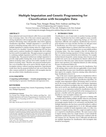
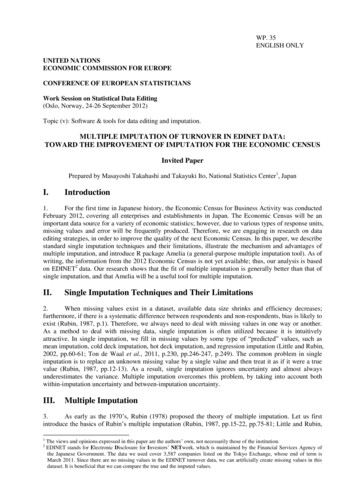
4randomly drawn from this observed sample of size n with replacement, and we repeat this process Mtimes.714.Figure 4.1 schematically shows multiple imputation, where M 5, using the EMB algorithm.First, there is incomplete data (sample size n), where q values are observed and n – q values are missing.Using the nonparametric bootstrapping method, a bootstrap subsample of size n is drawn from thisincomplete data M times (here, five times). We, then, apply the EM algorithm to each of these Mbootstrap subsamples, calculate M point estimates of and , impute missing values by M equations ofequation (3), and construct M multiply-imputed datasets. Using these M multiply-imputed datasetsseparately, we conduct statistical analysis and combine the results by equation (1) into the final results(Honaker and King, 2010, p.565; Congdon, 2006, p.504).Figure 4.1: Multiple Imputation via the EMB AlgorithmSource: Honaker, King, and Blackwell (2011, p.4)V.R Package Amelia II15.In the late 1970’s, Rubin (1978) proposed the theory of multiple imputation. Despite itstheoretical beauty, multiple imputation was computationally challenging, and it had not been used for solong in practice. In a social science field during the late 1990’s, about 94% of the journal articles usedlist-wise deletion to deal with missing data. In light of such reality in the social sciences, a team led byHarvard University Professor Gary King developed general-purpose multiple imputation software,Amelia8 (King et al., 2001). Since then, ten years have passed. Amelia has been used in many socialscience fields, but in order to accommodate the needs to apply multiple imputation to a gigantic dataset, itwas reborn as Amelia II, implemented with the new EMB Algorithm (Honaker and King, 2010).9 Asreported in Honaker and King (2010, p.565), Amelia II can handle 240 variables and 32,000 observations,i.e., 7.68 million variable-observations.16.There are two assumptions in Amelia II (Honaker, King, and Blackwell, 2011, p.3). First, thetheoretical true complete data are a multivariate normal distribution, which is often used as anapproximation to the true data distribution. By way of transformation, the distributions of many variables7Generally, the estimate based on bootstrap subsamples is less biased than the estimate based on the original sample. Also, as nand M go to infinity, the variance of bootstrap subsamples becomes a consistent estimate (Little and Rubin, 2002, p.80).8Amelia is named after an American female aviator, Amelia Earhart, who successfully flew over the Atlantic Ocean for the firsttime in history as a female aviator. In July 1937, during the around-the-world flight, she became missing, and her whereaboutsare still considered a mystery. With her fabulous career, she is still a legendary female aviator in the United States of America.9Amelia II can be downloaded from the following websites and can be implemented in R for free:http://gking.harvard.edu/amelia/ or http://cran.r-project.org/web/packages/Amelia/For software issues on multiple imputation, see Yucel (2011), Schmidt (2009), and Drechsler (2009).
5can be made realistically similar to a normal distribution. Second, missingness is either MAR or MCAR.Therefore, if missingness is NI, a specific method is called for. About a specific way to deal with missingdata, please refer to King et al. (2001, pp.65-66), which is out of the scope in this research.17.Assuming that Amelia II has already been downloaded and installed on the computer, let usbriefly explain Amelia functions.10 First, start Amelia II, using the library function.library(Amelia)18.Next, we should set the starting value, using the set.seed function. Amelia II utilizesbootstrapping; thus, if we do not set the seed, imputed values will become always different.11set.seed(1223)19.The amelia function is used to perform multiple imputation as follows. Here, a.out is anarbitrary variable name to store the results of multiple imputation, data is the name of the data we areusing, and the right hand side of m refers to the number of multiply-imputed datasets.a.out - amelia(data, m 5)20.Using the write.amelia function, the multiply-imputed datasets can be saved as a csv file.write.amelia(obj a.out, file.stem "outdata")21.While it is possible to conduct statistical analysis using the M separate datasets by hand, it isfortunate that R has another package called Zelig to perform this task more easily.12require("Zelig")z.out -zelig(Y X,data a.out imputations,model "ls",cite F)summary(z.out)print(summary(z.out), subset 1:3)VI.Multiple Imputation of Turnover in EDINET DataA.Descriptions of DatasetTable 6.1: Summary Statistics (Raw Data)VariableTurnover (E)Worker (E)Turnover (I)Worker (I)Turnover (D)Worker (D)Turnover (G)Worker (G)Turnover (L)Worker 705055720248673330906992911053150822.The data we used are based on EDINET data (Sectors E manufacturing, I retailing, D construction, G communication, and L service). Our dataset has two variables. One is Turnover (unit million yen), which is our dependent variable. The other is Worker (unit person), which is ourindependent variable. Our intuition suggests that as the number of workers increases, the amount ofturnover also increases. In the original dataset, there are no missing values in both variables, which meansthat we know the true values in these variables. For the purpose of experiment, we will artificially create10For more information on Amelia II, see Honaker, King, and Blackwell (2012a) and Honaker, King, and Blackwell (2012b).Philosophically, random numbers should become different, every time they are generated. However, the retaining ofreproducibility is important in scientific analyses; thus, we often retain reproducibility of random numbers by setting the seed.Nonetheless, if we repeatedly use the same ―random‖ number, it is no longer random, so that we have to be careful about how aspecific seed affects the results we obtain. If a specific seed generates a skewed dataset, using this seed cannot berecommended. Since Amelia assumes a normal distribution, it can be said that a seed that can generate an exact normaldistribution is a good seed. In R, we generated random samples of size 1000, using set.seed (1) to set.seed (5000), andchecked skewness, kurtosis, the Jarque-Bera test, and kernel densities. Among the 5000 seeds, we found that the following canbe recommended: 43, 393, 864, 1223, 1403, 1712, 1992, 2725, 2748, and 2902. Our analysis is based on set.seed (1223).12For more information on Zelig, see Honaker, King, and Blackwell (2011, pp.35-36) and Imai, King, and Lau (2008).11
6missing values in the Turnover variable. The models we used are first-order polynomial and naturallogarithm transformation. Summary statistics in raw data are presented in Table 6.1.23.Figures 6.1 and 6.2 show the histograms of Turnover and Worker in raw data for Sector E,respectively. Figure 6.3 shows the scatterplot between Turnover and Worker in raw data for Sector E.Figure 6.1: Turnover (Raw)24.Figure 6.2: Worker (Raw)Figure 6.3 (Raw, r 0.682)Summary statistics in log are presented in Table 6.2.Table 6.2: Summary Statistics (Natural Log)VariableObservationTurnover (E)Worker (E)Turnover (I)Worker (I)Turnover (D)Worker (D)Turnover (G)Worker (G)Turnover (L)Worker 71.3092.0231.34225.Figures 6.4 and 6.5 show the histograms of Turnover and Worker in log for Sector E,respectively. Figure 6.6 shows the scatterplot between Turnover and Worker in log for Sector E.Figure 6.4: Turnover (Log)B.Figure 6.5: Worker (Log)Figure 6.6 (Log, r 0.593)Assumptions of Missing Mechanism26.We created the following six patterns of missing mechanisms to cover both MCAR and MAR,but not NI: (1) Completely Random sampling (MCAR); (2) Turnover is missing if worker size is small(MAR); (3) Turnover is missing if worker size is medium (MAR); (4) Turnover is missing if worker sizeis large (MAR); (5) Turnover is missing if worker size is small or large (MAR); (6) Systematic sampling(MAR). The percentage of missing values in the dataset is 30%, 40%, and 50%. Therefore, there are 18patterns of missingness in our experiment.
7Figure 6.7: MCAR (50%)C.Figure 6.8: MAR (50%, Worker Small)Figure 6.9: MAR (50%, Worker Medium)Results of Multiple Imputation and Single Imputation27.We compared the true values of Turnover with the imputed values from multiple imputation andsingle imputation, respectively. Table 6.3 shows the results of these comparisons. For instance, in sectorE (manufacturing), the difference between the true values and the multiply-imputed values is generally(66.7%) less than the difference between the true values and the singly-imputed values. In Sector I(retailing), the difference between the true values and the multiply-imputed values is the same (50%) asthe difference between the true values and the singly-imputed values, etc. Overall, in the EDINET data,multiple imputation is closer to the true values than single imputation, 62.5 times out of 100.Table 6.3SectorE (n 1222, manufacturing)I (n 571, retailing)D (n 158, construction)G (n 276, communication)L (n 191, service)TotalMultiple Imputation66.7%50.0%10.0%85.7%92.3%62.5%Single Imputation33.3%50.0%90.0%14.3%7.7%37.5%Total100 %100 %100 %100 %100 %100 %28.Table 6.4 shows the comparisons across missing patterns. For instance, when the missing patternis completely random, the difference between the true values and the multiply-imputed values isgenerally (75%) less than the difference between the true values and the singly-imputed values, etc.Table 6.4Missing PatternCompletely RandomWorker Size SmallWorker Size MediumWorker Size LargeWorker Size Large & SmallSystematic SamplingMultiple Imputation75.0%75.0%90.0%66.7%50.0%20.0%Single Imputation25.0%25.0%10.0%33.3%50.0%80.0%Total100 %100 %100 %100 %100 %100 %29.Table 6.5 shows that, in both models (1st order polynomial and logarithm), multiple imputationoutperforms single imputation (64.7% and 60.9%, respectively).Table 6.5Models1st Order PolynomialNatural LogMultiple Imputation64.7%60.9%Single Imputation35.3%39.1%Total100 %100 %30.Table 6.6 shows that, the higher the rate of missingness, the more multiple imputationoutperforms single imputation (55.0%, 69.2%, and 71.4%, respectively).
8Table 6.6Missing Rate30%40%50%Multiple Imputation55.0%69.2%71.4%Single Imputation45.0%30.8%28.6%Total100 %100 %100 %31.In the following, due to the limited space, we only show the results of missing patterns (1) and(2) in the 50% missingness setting, using log transformed data for Sector E. The number of multiplyimputed datasets, M, is set to 20. For the choice of M, see Rubin (1987, p.114) and Schafer (1999, p.7).Our results for multiple imputation are based on the average of the 20 multiply-imputed datasets.32.In the case of MCAR, the standard deviation of the true values (log) is 1.532. The standarddeviation of the multiply-imputed values (log) is 1.525, while the standard deviation of the singlyimputed values (log) is 0.889. Therefore, the true standard deviation is better estimated by multipleimputation than by single imputation. Figure 6.10 shows the scatterplot between Turnover and Worker,including both observed values and singly-imputed values (red circles). Figures 6.11a and 6.11b show thescatterplots between Turnover and Worker, including both observed values and multiply-imputed values(red circles) for m 1 and m 10. As visible, the singly-imputed values form a single, straight line,which means that it underestimates the variance, while the multiply-imputed values are scattered just asthe true values shown in Figure 6.6.Figure 6.6:True Scatterplot in LogFigure 6.10:Single Imputation (MCAR)Figure 6.11a:Multiple Imputation (m 1)Figure 6.11b:Multiple Imputation (m 10)33.In the above, we compared the true values and the imputed values. For the purpose of experiment,this is the most accurate way of evaluating the performance of imputation models; however, in reality,true values are always unknown. Therefore, the fit of imputation models can never be directly tested inreality. As a result, the diagnostic methods in imputation had long been ignored. Nonetheless, Abayomi,Gelman, and Levy (2008) show that the fit of imputation models and the assumptions of missingmechanisms can be indirectly tested. Amelia II supplies the ―comparing densities‖ function, the―overimpute‖ function, the ―overdispersed starting values‖ function, and the ―missingness map‖ function(Honaker, King, and Blackwell, 2011, pp.25-35). In the ―comparing densities‖ function, we compare thedensities of observed values and imputed values. If the two densities are almost the same, it is likely thatthe imputation model is free of problems. In the ―overimpute‖ function, we sequentially impute eachobserved value as if they were missing and then construct 90% confidence intervals. In the―overdispersed starting values‖ function, we set various starting values for the EM algorithm to see if allof the starting values converge to the same value. In the ―missingness‖ map function, we can visualize thepattern of missingness in the dataset.34.Suppose that we do not know the true values. We can still diagnose the fit of multiple imputation,using the above mentioned diagnostic techniques. Figure 6.12 compares the densities of observed valuesand imputed values in the case of missing mechanism (1), i.e., completely random. We can see that thetwo densities are reasonably similar; thus, we can conclude that the imputation model fits very well.Figure 6.13 shows the missingness map, where Worker is in an increasing order. We see no discerniblepatterns in Turnover; therefore, we can infer that the missing mechanism is MCAR. Since we createdthese missing values ourselves, we know that these diagnostics are actually correct. In Figure 6.14, wesee that the imputation model is generally captured by the 90% confidence interval. Figure 6.15 showsthat all of the starting values for the EM algorithm converged to the same value.
9Figure 6.12:Densities (MCAR)Figure 6.13:Missingness Map (MCAR)Figure 6.14:Overimputation (MCAR)Figure 6.15: OverdispersedStarting Values (MCAR)35.In the case of missing mechanism (2), i.e., MAR (Worker Small), the standard deviation of thetrue values (log) is 1.240. The standard deviation of the multiply-imputed values (log) is 1.426, while thestandard deviation of the singly-imputed values (log) is 0.736. Therefore, the true standard deviation is,again, better estimated by multiple imputation than by single imputation. Figure 6.16 shows thescatterplot between Turnover and Worker, including both observed values and singly-imputed values (redcircles). Figures 6.17a and 6.17b show the scatterplots between Turnover and Worker, including bothobserved values and multiply-imputed values (red circles) for m 1 and m 10. As visible, the singlyimputed values, once again, form a single, straight line, which means that it underestimates the variance,while the multiply-imputed values are scattered just as the true values shown in Figure 6.6.Figure 6.6:True Scatterplot in LogFigure 6.16:Single Imputation (MAR)Figure 6.17a:Multiple Imputation (m 1)Figure 6.17b:Multiple Imputation (m 10)36.Figure 6.18 compares the densities of observed values and imputed values in the case of MAR.We can see that the two densities are drastically different. When the two densities are different, this doesnot automatically mean that the imputation model is wrong. This simply implies that we should look intothe details to find out why the two densities are different. Figure 6.19 shows the missingness map, whereWorker is in an increasing order. We see discernible patterns in Turnover; therefore, we can infer that themissing mechanism is MAR. Thus, we now infer that the density of missing values should be differentfrom the density of observed values, so that Figure 6.18 should not be considered problematic. Again, weknow that these diagnostics are, in fact, correct. In Figure 6.20, we see that the imputation model isgenerally captured by the 90% confidence interval. Figure 6.21 shows that all of the starting values forthe EM algorithm converged to the same value.Figure 6.18:Densities (MAR)Figure 6.19:Missingness Map (MAR)Figure 6.20:Overimputation (MAR)Figure 6.21: OverdispersedStarting Values (MAR)
10VII. Conclusions and Future Research37.This research shows that the overall fit of multiple imputation is excellent, and that it is anefficient method of imputation. Also, we found that R package Amelia II is a useful program for multipleimputation. However, there is no single perfect method to impute missing values, and each imputationmethod has its own advantages and disadvantages. Even multiple imputation is no exceptions, and if theassumptions are drastically wrong, then the accuracy of imputation cannot be guaranteed. The diagnosticmethods in multiple imputation that are shown in this paper are still under development. We diagnosedthe M combined results, but there is no way of diagnosing each of the M multiply imputed datasets, as ofwriting. In order to guarantee the accuracy of multiply-imputed datasets in practice, for future research,the diagnostic methods should be further developed. Also, in this research, we did not take the existenceof outliers in EDINET data into account. However, the accuracy of regression models is largelydependent on the influence of outliers. Thus, in future research, we will consider the impact of outliers onimputation. R package VIM allows us to investigate the missingness structure in a dataset and is expectedto be useful for the purpose of diagnostics (Templ, Kowarik, and Filzmoser, 5.16.17.18.19.20.21.22.23.24.25.26.Abayomi, Kobi, Andrew Gelman, and Marc Levy. (2008). ―Diagnostics for Multivariate Imputations,‖ Applied Statisticsvol.57, no.3: 273-291.Congdon, Peter. (2006). Bayesian Statistical Modelling, Second Edition. West Sussex: John Wiley & Sons Ltd.DeGroot, Morris H. and Mark J. Schervish. (2002). Probability and Statistics. Boston: Addison-Wesley.Drechsler, Jörg. (2009). ―Far From Normal - Multiple Imputation of Missing Values in a German Establishment Survey,‖Work Session on Statistical Data Editing, Conferenc
4 randomly drawn from this observed sample of size n with replacement, and we repeat this process M times.7 14. Figure 4.1 schematically shows multiple imputation, where M 5, using the EMB algorithm. First, there is incomplete data (sample size n), where q values are observed and n - q values are missing. Using the nonparametric bootstrapping method, a bootstrap subsample of size n is .