Transcription
JSSJournal of Statistical SoftwareDecember 2011, Volume 45, Issue 3.http://www.jstatsoft.org/mice: Multivariate Imputation by ChainedEquations in RStef van BuurenKarin Groothuis-OudshoornTNOUniversity of TwenteAbstractThe R package mice imputes incomplete multivariate data by chained equations. Thesoftware mice 1.0 appeared in the year 2000 as an S-PLUS library, and in 2001 as anR package. mice 1.0 introduced predictor selection, passive imputation and automaticpooling. This article documents mice 2.9, which extends the functionality of mice 1.0in several ways. In mice 2.9, the analysis of imputed data is made completely general,whereas the range of models under which pooling works is substantially extended. mice 2.9adds new functionality for imputing multilevel data, automatic predictor selection, datahandling, post-processing imputed values, specialized pooling routines, model selectiontools, and diagnostic graphs. Imputation of categorical data is improved in order to bypassproblems caused by perfect prediction. Special attention is paid to transformations, sumscores, indices and interactions using passive imputation, and to the proper setup ofthe predictor matrix. mice 2.9 can be downloaded from the Comprehensive R ArchiveNetwork. This article provides a hands-on, stepwise approach to solve applied incompletedata problems.Keywords: MICE, multiple imputation, chained equations, fully conditional specification,Gibbs sampler, predictor selection, passive imputation, R.1. IntroductionMultiple imputation (Rubin 1987, 1996) is the method of choice for complex incomplete dataproblems. Missing data that occur in more than one variable presents a special challenge.Two general approaches for imputing multivariate data have emerged: joint modeling (JM)and fully conditional specification (FCS), also known as multivariate imputation by chainedequations (MICE). Schafer (1997) developed various JM techniques for imputation under themultivariate normal, the log-linear, and the general location model. JM involves specifying amultivariate distribution for the missing data, and drawing imputation from their conditional
2mice: Multivariate Imputation by Chained Equations in Rdistributions by Markov chain Monte Carlo (MCMC) techniques. This methodology is attractive if the multivariate distribution is a reasonable description of the data. FCS specifies themultivariate imputation model on a variable-by-variable basis by a set of conditional densities,one for each incomplete variable. Starting from an initial imputation, FCS draws imputationsby iterating over the conditional densities. A low number of iterations (say 10–20) is oftensufficient. FCS is attractive as an alternative to JM in cases where no suitable multivariatedistribution can be found. The basic idea of FCS is already quite old, and has been proposedusing a variety of names: stochastic relaxation (Kennickell 1991), variable-by-variable imputation (Brand 1999), regression switching (van Buuren et al. 1999), sequential regressions(Raghunathan et al. 2001), ordered pseudo-Gibbs sampler (Heckerman et al. 2001), partiallyincompatible MCMC (Rubin 2003), iterated univariate imputation (Gelman 2004), MICE(van Buuren and Oudshoorn 2000; van Buuren and Groothuis-Oudshoorn 2011) and FCS(van Buuren 2007).Software implementationsSeveral authors have implemented fully conditionally specified models for imputation. mice 1.0(van Buuren and Oudshoorn 2000) was released as an S-PLUS library in 2000, and was converted by several users into R (R Development Core Team 2011). IVEware (Raghunathanet al. 2001) is a SAS-based procedure that was independently developed by Raghunathan andcolleagues. The function aRegImpute in R and S-PLUS is part of the Hmisc package (Harrell2001). The ice software (Royston 2004, 2005; Royston and White 2011) is a widely usedimplementation in Stata. SOLAS 3.0 (Statistical Solutions 2001) is also based on conditionalspecification, but does not iterate. WinMICE (Jacobusse 2005) is a Windows stand-aloneprogram for generating imputations under the hierarchical linear model. A recent additionis the R package mi (Su et al. 2011). Furthermore, FCS is now widely available throughthe multiple imputation procedure part of the SPSS 17 Missing Values Analysis add-onmodule. See http://www.multiple-imputation.com/ for an overview.Applications of chained equationsApplications of imputation by chained equations have now appeared in quite diverse fields:addiction (Schnoll et al. 2006; MacLeod et al. 2008; Adamczyk and Palmer 2008; Caria et al.2009; Morgenstern et al. 2009), arthritis and rheumatology (Wolfe et al. 2006; Rahman et al.2008; van den Hout et al. 2009), atherosclerosis (Tiemeier et al. 2004; van Oijen et al. 2007;McClelland et al. 2008), cardiovascular system (Ambler et al. 2005; van Buuren et al. 2006a;Chase et al. 2008; Byrne et al. 2009; Klein et al. 2009), cancer (Clark et al. 2001, 2003; Clarkand Altman 2003; Royston et al. 2004; Barosi et al. 2007; Fernandes et al. 2008; Sharma et al.2008; McCaul et al. 2008; Huo et al. 2008; Gerestein et al. 2009), epidemiology (Cummingset al. 2006; Hindorff et al. 2008; Mueller et al. 2008; Ton et al. 2009), endocrinology (Rouxelet al. 2004; Prompers et al. 2008), infectious diseases (Cottrell et al. 2005; Walker et al.2006; Cottrell et al. 2007; Kekitiinwa et al. 2008; Nash et al. 2008; Sabin et al. 2008; Theinet al. 2008; Garabed et al. 2008; Michel et al. 2009), genetics (Souverein et al. 2006), healtheconomics (Briggs et al. 2003; Burton et al. 2007; Klein et al. 2008; Marshall et al. 2009),obesity and physical activity (Orsini et al. 2008a; Wiles et al. 2008; Orsini et al. 2008b; vanVlierberghe et al. 2009), pediatrics and child development (Hill et al. 2004; Mumtaz et al.2007; Deave et al. 2008; Samant et al. 2008; Butler and Heron 2008; Ramchandani et al.2008; van Wouwe et al. 2009), rehabilitation (van der Hulst et al. 2008), behavior (Veenstra
Journal of Statistical Software3et al. 2005; Melhem et al. 2007; Horwood et al. 2008; Rubin et al. 2008), quality of care (Sisket al. 2006; Roudsari et al. 2007; Ward and Franks 2007; Grote et al. 2007; Roudsari et al.2008; Grote et al. 2008; Sommer et al. 2009), human reproduction (Smith et al. 2004a,b;Hille et al. 2005; Alati et al. 2006; O’Callaghan et al. 2006; Hille et al. 2007; Hartog et al.2008), management sciences (Jensen and Roy 2008), occupational health (Heymans et al.2007; Brunner et al. 2007; Chamberlain et al. 2008), politics (Tanasoiu and Colonescu 2008),psychology (Sundell et al. 2008) and sociology (Finke and Adamczyk 2008). All authors usesome form of chained equations to handle the missing data, but the details vary considerably.The interested reader could check out articles from a familiar application area to see howmultiple imputation is done and reported.FeaturesThis paper describes the R package mice 2.9 for multiple imputation: generating multipleimputation, analyzing imputed data, and for pooling analysis results. Specific features of thesoftware are: Columnwise specification of the imputation model (Section 3.2). Arbitrary patterns of missing data (Section 6.2). Passive imputation (Section 3.4). Subset selection of predictors (Section 3.3). Support of arbitrary complete-data methods (Section 5.1). Support pooling various types of statistics (Section 5.3). Diagnostics of imputations (Section 4.5). Callable user-written imputation functions (Section 6.1).Package mice 2.9 replaces version mice 1.21, but is compatible with previous versions. Thisdocument replaces the original manual (van Buuren and Oudshoorn 2000). The mice 2.9package extends mice 1.0 in several ways. New features in mice 2.9 include: quickpred() for automatic generation of the predictor matrix (Section 3.3). mice.impute.2L.norm() for imputing multilevel data (Section 3.3). Stable imputation of categorical data (Section 4.4). Post-processing imputations through the post argument (Section 3.5). with.mids() for general data analysis on imputed data (Section 5.1). pool.scalar() and pool.r.squared() for specialized pooling (Section 5.3). pool.compare() for model testing on imputed data (Section 5.3). cbind.mids(), rbind.mids() and ibind() for combining imputed data (see help fileof these functions).
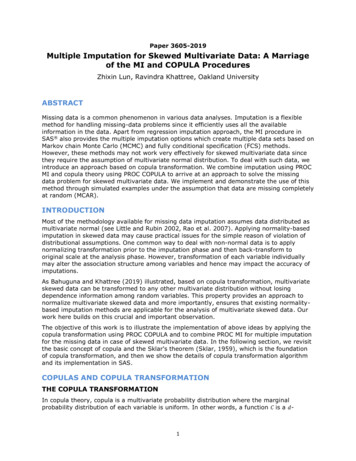
4mice: Multivariate Imputation by Chained Equations in RFurthermore, this document introduces a new strategy to specify the predictor matrix inconjunction with passive imputation. The amount and scope of example code has beenexpanded considerably. All programming code used in this paper is available in the filev45i03.R along with the manuscript and as doc/JSScode.R in the mice package.The intended audience of this paper consists of applied researchers who want to address problems caused by missing data by multiple imputation. The text assumes basic familiarity withR. The document contains hands-on analysis using the mice package. We do not discuss problems of incomplete data in general. We refer to the excellent books by Little and Rubin (2002)and Schafer (1997). Theory and applications of multiple imputation have been developed inRubin (1987) and Rubin (1996). van Buuren (2012) introduces multiple imputation from anapplied perspective.Package mice 2.9 was written in pure R using old-style S3 classes and methods. mice 2.9 waswritten and tested in R 2.12.2. The package has a simple architecture, is highly modular, andallows easy access to all program code from within the R environment.2. General frameworkTo the uninitiated, multiple imputation is a bewildering technique that differs substantiallyfrom conventional statistical approaches. As a result, the first-time user may get lost ina labyrinth of imputation models, missing data mechanisms, multiple versions of the data,pooling, and so on. This section describes a modular approach to multiple imputation thatforms the basis of the architecture of mice. The philosophy behind the MICE methodology isthat multiple imputation is best done as a sequence of small steps, each of which may requirediagnostic checking. Our hope is that the framework will aid the user to map out the stepsneeded in practical applications.2.1. NotationLet Yj with (j 1, . . . , p) be one of p incomplete variables, where Y (Y1 , . . . , Yp ). Theobserved and missing parts of Yj are denoted by Yjobs and Yjmis , respectively, so Y obs (Y1obs , . . . , Ypobs ) and Y mis (Y1mis , . . . , Ypmis ) stand for the observed and missing data in Y .The number of imputation is equal to m 1. The hth imputed data sets is denoted as Y (h)where h 1, . . . , m. Let Y j (Y1 , . . . , Yj 1 , Yj 1 , . . . , Yp ) denote the collection of the p 1variables in Y except Yj . Let Q denote the quantity of scientific interest (e.g., a regressioncoefficient). In practice, Q is often a multivariate vector. More generally, Q encompasses anymodel of scientific interest.2.2. Modular approach to multiple imputationFigure 1 illustrates the three main steps in multiple imputation: imputation, analysis andpooling. The software stores the results of each step in a specific class: mids, mira and mipo.We now explain each of these in more detail.The leftmost side of the picture indicates that the analysis starts with an observed, incomplete data set Yobs . In general, the problem is that we cannot estimate Q from Yobs withoutmaking unrealistic assumptions about the unobserved data. Multiple imputation is a generalframework that several imputed versions of the data by replacing the missing values by plau-
Journal of Statistical Softwareincomplete dataimputed datamice()data frame5analysis resultswith()midspooled resultspool()miramipoFigure 1: Main steps used in multiple imputation.sible data values. These plausible values are drawn from a distribution specifically modeledfor each missing entry. In mice this task is being done by the function mice(). Figure 1portrays m 3 imputed data sets Y (1) , . . . , Y (3) . The three imputed sets are identical for thenon-missing data entries, but differ in the imputed values. The magnitude of these differencereflects our uncertainty about what value to impute. The package has a special class forstoring the imputed data: a multiply imputed dataset of class mids.The second step is to estimate Q on each imputed data set, typically by the method wewould have used if the data had been complete. This is easy since all data are now complete. The model applied to Y (1) , . . . , Y (m) is the generally identical. mice 2.9 contains afunction with.mids() that perform this analysis. This function supersedes the lm.mids()and glm.mids(). The estimates Q̂(1) , . . . , Q̂(m) will differ from each other because their inputdata differ. It is important to realize that these differences are caused because of our uncertainty about what value to impute. In mice the analysis results are collectively stored as amultiply imputed repeated analysis within an R object of class mira.The last step is to pool the m estimates Q̂(1) , . . . , Q̂(m) into one estimate Q̄ and estimate itsvariance. For quantities Q that are approximately normally distributed, we can calculate themean over Q̂(1) , . . . , Q̂(m) and sum the within- and between-imputation variance accordingto the method outlined in Rubin (1987, pp. 76–77). The function pool() contains methodsfor pooling quantities by Rubin’s rules. The results of the function is stored as a multipleimputed pooled outcomes object of class mipo.2.3. MICE algorithmThe imputation model should Account for the process that created the missing data. Preserve the relations in the data. Preserve the uncertainty about these relations.The hope is that adherence to these principles will yield imputations that are statistically
6mice: Multivariate Imputation by Chained Equations in Rcorrect as in Rubin (1987, Chapter 4) for a wide range in Q. Typical problems that maysurface while imputing multivariate missing data are For a given Yj , predictors Y j used in the imputation model may themselves be incomplete. Circular dependence can occur, where Y1 depends on Y2 and Y2 depends on Y1 becausein general Y1 and Y2 are correlated, even given other variables. Especially with large p and small n, collinearity and empty cells may occur. Rows or columns can be ordered, e.g., as with longitudinal data. Variables can be of different types (e.g., binary, unordered, ordered, continuous), therebymaking the application of theoretically convenient models, such as the multivariatenormal, theoretically inappropriate. The relation between Yj and Y j could be complex, e.g., nonlinear, or subject to censoring processes. Imputation can create impossible combinations (e.g., pregnant fathers), or destroy deterministic relations in the data (e.g., sum scores). Imputations can be nonsensical (e.g., body temperature of the dead). Models for Q that will be applied to the imputed data may not (yet) be known.This list is by no means exhaustive, and other complexities may appear for particular data.In order to address the issues posed by the real-life complexities of the data, it is convenientto specify the imputation model separately for each column in the data. This has led by tothe development of the technique of chained equations. Specification occurs on at a level thatis well understood by the user, i.e., at the variable level. Moreover, techniques for creatingunivariate imputations have been well developed.Let the hypothetically complete data Y be a partially observed random sample from the pvariate multivariate distribution P (Y θ). We assume that the multivariate distribution of Yis completely specified by θ, a vector of unknown parameters. The problem is how to get themultivariate distribution of θ, either explicitly or implicitly. The MICE algorithm obtains theposterior distribution of θ by sampling iteratively from conditional distributions of the formP (Y1 Y 1 , θ1 ).P (Yp Y p , θp ).The parameters θ1 , . . . , θp are specific to the respective conditional densities and are notnecessarily the product of a factorization of the ‘true’ joint distribution P (Y θ). Starting froma simple draw from observed marginal distributions, the tth iteration of chained equations isa Gibbs sampler that successively draws (t)θ1(t 1) P (θ1 Y1obs , Y2, . . . , Yp(t 1) )
Journal of Statistical Software (t)Y1(t 1) P (Y1 Y1obs , Y2.(t)7 (t), . . . , Yp(t 1) , θ1 )(t)θp (t) P (θp Ypobs , Y1 , . . . , Yp 1 )(t)Yp (t) P (Yp Ypobs , Y1 , . . . , Yp(t) , θp (t) )(t)where Yj (t) (Yjobs , Yj (t 1)Yj) is the jth imputed variable at iteration t. Observe that previous (t)imputationsonly enter Yj through its relation with other variables, and not directly.Convergence can therefore be quite fast, unlike many other MCMC methods. It is importantto monitor convergence, but in our experience the number of iterations can often be a smallnumber, say 10–20. The name chained equations refers to the fact that the MICE algorithmcan be easily implemented as a concatenation of univariate procedures to fill out the missingdata. The mice() function executes m streams in parallel, each of which generates oneimputed data set.The MICE algorithm possesses a touch of magic. The method has been found to work wellin a variety of simulation studies (Brand 1999; Horton and Lipsitz 2001; Moons et al. 2006;van Buuren et al. 2006b; Horton and Kleinman 2007; Yu et al. 2007; Schunk 2008; Drechslerand Rassler 2008; Giorgi et al. 2008). Note that it is possible to specify models for whichno known joint distribution exits. Two linear regressions specify a joint multivariate normalgiven specific regularity condition (Arnold and Press 1989). However, the joint distributionof one linear and, say, one proportional odds regression model is unknown, yet very easy tospecify with the MICE framework. The conditionally specified model may be incompatiblein the sense that the joint distribution cannot exist. It is not yet clear what the consequencesof incompatibility are on the quality of the imputations. The little simulation work that isavailable suggests that the problem is probably not serious in practice (van Buuren et al.2006b; Drechsler and Rassler 2008). Compatible multivariate imputation models (Schafer1997) have been found to work in a large variety of cases, but may lack flexibility to address specific features of the data. Gelman and Raghunathan (2001) remark that “separateregressions often make more sense than joint models”. In order to bypass the limitationsof joint models, Gelman (2004, pp. 541) concludes: “Thus we are suggesting the use of anew class of models—inconsistent conditional distributions—that were initially motivated bycomputational and analytical convenience.” As a safeguard to evade potential problems byincompatibility, we suggest that the order in which variable are imputed should be sensible.This ordering can be specified in mice (cf. Section 3.6). Existence and uniqueness theoremsfor conditionally specified models have been derived (Arnold and Press 1989; Arnold et al.1999; Ip and Wang 2009). More work along these lines would be useful in order to identifythe boundaries at which the MICE algorithm breaks down. Barring this, the method seemsto work well in many examples, is of great importance in practice, and is easily applied.2.4. Simple exampleThe section presents a simple example incorporating all three steps. After installing theR package mice from the Comprehensive R Archive Network (CRAN), load the package.R library("mice")This paper uses the features of mice 2.9. The data frame nhanes contains data from Schafer
8mice: Multivariate Imputation by Chained Equations in R(1997, p. 237). The data contains four variables: age (age group), bmi (body mass index),hyp (hypertension status) and chl (cholesterol level). The data are stored as a data frame.Missing values are represented as NA.R nhanes12345age bmi hyp chl1NA NA NA2 22.71 1871NA1 1873NA NA NA1 20.41 113.Inspecting the missing dataThe number of the missing values can be counted and visualized as follows:R md.pattern(nhanes)131317age hyp bmi chl1111 01101 11110 11001 21000 3089 10 27There are 13 (out of 25) rows that are complete. There is one row for which only bmi ismissing, and there are seven rows for which only age is known. The total number of missingvalues is equal to (7 3) (1 2) (3 1) (1 1) 27. Most missing values (10) occurin chl.Another way to study the pattern involves calculating the number of observations per patternsfor all pairs of variables. A pair of variables can have exactly four missingness patterns: bothvariables are observed (pattern rr), the first variable is observed and the second variable ismissing (pattern rm), the first variable is missing and the second variable is observed (patternmr), and both are missing (pattern mm). We can use the md.pairs() function to calculate thefrequency in each pattern for all variable pairs asR p - md.pairs(nhanes)R p rrage bmi hyp chlage 25 16 17 15bmi 16 16 16 13
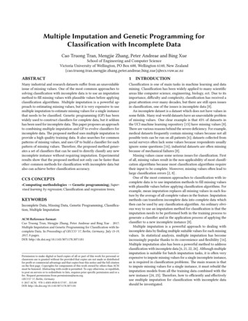
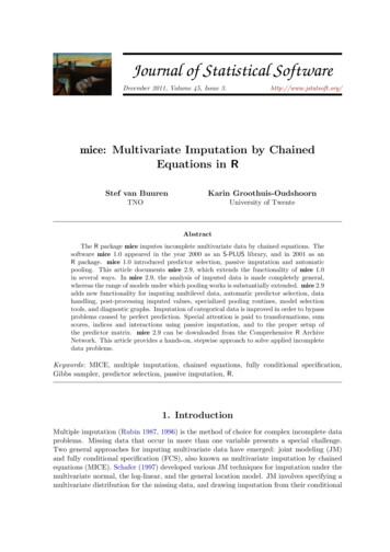
Journal of Statistical Softwarehypchl17151613171491415 rmagebmihypchlage bmi hyp chl098 10000301030210 mragebmihypchlage bmi hyp chl00009012800110330 mmagebmihypchlage bmi hyp chl000009870887077 10Thus, for pair (bmi,chl) there are 13 completely observed pairs, 3 pairs for which bmi isobserved but hyp not, 2 pairs for which bmi is missing but with hyp observed, and 7 pairswith both missing bmi and hyp. Note that these numbers add up to the total sample size.The R package VIM (Templ et al. 2011) contains functions for plotting incomplete data. Themargin plot of the pair (bmi,chl) can be plotted byR library("VIM")R marginplot(nhanes[, c("chl", "bmi")], col mdc(1:2), cex 1.2, cex.lab 1.2, cex.numbers 1.3, pch 19)Figure 2 displays the result. The data area holds 13 blue points for which both bmi and chlwere observed. The plot in Figure 2 requires a graphic device that supports transparentcolors, e.g., pdf(). To create the plot in other devices, change the col mdc(1:2) argumentto col mdc(1:2, trans FALSE). The three red dots in the left margin correspond tothe records for which bmi is observed and chl is missing. The points are drawn at the knownvalues of bmi at 24.9, 25.5 and 29.6. Likewise, the bottom margin contain two red points withobserved chl and missing bmi. The red dot at the intersection of the bottom and left marginindicates that there are records for which both bmi and chl are missing. The three numbersat the lower left corner indicate the number of incomplete records for various combinations.There are 9 records in which bmi is missing, 10 records in which chl is missing, and 7 recordsin which both are missing. Furthermore, the left margin contain two box plots, a blue anda red one. The blue box plot in the left margin summarizes the marginal distribution of bmiof the 13 blue points. The red box plot summarizes the distribution of the three bmi values
mice: Multivariate Imputation by Chained Equations in R2025bmi30351097 150200250chlFigure 2: Margin plot of bmi versus chl as drawn by the marginplot() function in the VIMpackage. Observed data in blue, missing data in red.with missing chl. Under MCAR, these distribution are expected to be identical. Likewise,the two colored box plots in the bottom margin summarize the respective distributions forchl.Creating imputationsCreating imputations can be done with a call to mice() as follows:R imp - mice(nhanes, seed 23109)iter imp variable11 bmi hyp12 bmi hyp13 bmi hyp14 bmi hyp15 bmi hyp21 bmi hyp22 bmi hyp.chlchlchlchlchlchlchlwhere the multiply imputed data set is stored in the object imp of class mids. Inspect whatthe result looks likeR print(imp)
Journal of Statistical Software11Multiply imputed data setCall:mice(data nhanes, seed 23109)Number of multiple imputations: 5Missing cells per column:age bmi hyp chl098 10Imputation methods:agebmihypchl"" "pmm" "pmm" "pmm"VisitSequence:bmi hyp chl234PredictorMatrix:age bmi hyp chlage0000bmi1011hyp1101chl1110Random generator seed value: 23109Imputations are generated according to the default method, which is, for numerical data, predictive mean matching (pmm). The entries imp VisitSequence and imp PredictorMatrixare algorithmic options that will be discusses later. The default number of multiple imputations is equal to m 5.Diagnostic checkingAn important step in multiple imputation is to assess whether imputations are plausible.Imputations should be values that could have been obtained had they not been missing.Imputations should be close to the data. Data values that are clearly impossible (e.g., negativecounts, pregnant fathers) should not occur in the imputed data. Imputations should respectrelations between variables, and reflect the appropriate amount of uncertainty about their‘true’ values. Diagnostic checks on the imputed data provide a way to check the plausibilityof the imputations. The imputations for bmi are stored asR imp imp .0
12mice: Multivariate Imputation by Chained Equations in REach row corresponds to a missing entry in bmi. The columns contain the multiple imputations. The completed data set combines the observed and imputed values. The (first)completed data set can be obtained asR complete(imp)12345age12131.bmi hyp chl29.61 23822.71 18729.61 18720.41 18620.41 113The complete() function extracts the five imputed data sets from the imp object as a long(row-stacked) matrix with 125 records. The missing entries in nhanes have now been filled bythe values from the first (of five) imputation. The second completed data set can be obtainedby complete(imp, 2). For the observed data, it is identical to the first completed data set,but it may differ in the imputed data.It is often useful to inspect the distributions of original and the imputed data. One way ofdoing this is to use the function stripplot() in mice 2.9, an adapted version of the samefunction in the package lattice (Sarkar 2008). The stripplot in Figure 3 is created asR stripplot(imp, pch 20, cex 1.2)The figure shows the distributions of the four variables as individual points. Blue points areobserved, the red points are imputed. The panel for age contains blue points only becauseage is complete. Furthermore, note that the red points follow the blue points reasonably well,including the gaps in the distribution, e.g., for chl.The scatterplot of chl and bmi for each imputed data set in Figure 4 is created byR xyplot(imp, bmi chl .imp, pch 20, cex 1.4)The figure redraws figure 2, but now for the observed and imputed data. Imputations areplotted in red. The blue points are the same across different panels, but the red point vary.The red points have more or less the same shape as blue data, which indicates that they couldhave been plausible measurements if they had not been missing. The differences between thered points represents our uncertainty about the true (but unknown) values.Under MCAR, univariate distributions of the observed and imputed data are expected tobe identical. Under MAR, they can be different, both in location and spread, but theirmultivariate distribution is assumed to be identical. There are many other ways to look atthe completed data, but we defer of a discussion of those to Section 4.5.Analysis of imputed dataSuppose that the complete-data analysis of interest is a linear regression of chl on age andbmi. For this purpose, we can use the function with.mids(), a wrapper function that appliesthe complete data model to each of the imputed data sets:
Journal of Statistical tation numberFigure 3: Stripplot of four variables in the original data and in the five imputed data sets.Points are slightly jittered. Observed data in blue, imputed data in red.R fit - with(imp, lm(chl age bmi))The fit object has class mira and contains the results of five complete-data analyses. Thesecan be pooled as follows:R print(pool(fit))Call: pool(object fit)Pooled .212025Fraction of information about the coefficients missing due to 795427More detailed output can be obtained, as usual, with the summary() function, i.e.,R round(summary(pool(fit)), 2)
14mice: Multivariate Imputation by Chained Equations in 250chlFigure 4: Scatterplot of cholesterol (chl) and body mass index (bmi) in the original data(panel 0), and five imputed data sets. Observed data in blue, imputed data in red.estsetdf Pr( t )lo 95 hi 95 nmis fmi(Intercept) -34.16 76.07 -0.45 6.810.67 -215.05 146.73NA 0.57age34.33 14.86 2.31 4.040.08-6.76 75.420 0.75bmi6.21 2.21 2.81 8.800.021.20 11.239 0.48lambda(Intercept)0.47age0.65bmi0.37After multiple imputation, we find a significant effect bmi. The column fmi contains thefraction of missing information as defined in Rubin (1987), and the column lambda is theproportion of the total variance that is attributable to the missing data (λ (B B/m)/T ).The pooled results are subject to simulation error and therefore depend on the seed argumentof the mice() function. In order to minimize simulation error, we can use a higher numberof imputations, for example m 50. It is easy to do this asR imp50 - mice(nhanes, m 50, seed 23109)R fit - with(imp50, lm(chl age bmi))R round(summary(pool(fit)), 2)estsetdf Pr( t )lo 95 hi 95 nmis(Intercept) -35.53 63.61 -0.56 14.460.58 -171.55 100.49NAage35.90 10.48 3.42 12.760.0013.21 58.580bmi6.15 1.97 3.13 15.130.011.96 10.359
Journal of Statistical Software15fmi lambda(Intercept) 0.350.27age0.430.35bmi0.320.24We find t
Keywords: MICE, multiple imputation, chained equations, fully conditional speci cation, Gibbs sampler, predictor selection, passive imputation, R. 1. Introduction Multiple imputation (Rubin1987,1996) is the method of choice for complex incomplete data problems. Missing data that occur in more than one variable presents a special challenge.