WIXLIB

Volume MeasureStudyAggregate Share VolumeGallant, Rossi, and Tauchen(1992), Hiemstra and Jones(1994), Ying (1966)Individual Share VolumeAndersen (1996), Epps andEpps (1976), James andEdmister (1983), Lamoureux andLastrapes (1990, 1994)Aggregate Dollar Volume—Individual Dollar VolumeJames and Edmister (1983),Lakonishok and Vermaelen(1986)Relative Individual DollarVolumeTkac (1996)Individual TurnoverBamber (1986, 1987), Hu (1997),Lakonishok and Smidt (1986),Morse (1980), Richardson,Sefcik, Thompson (1986), Stickeland Verrechia (1994)Aggregate TurnoverCampbell, Grossman, Wang(1993), LeBaron (1992), Smidt(1990), NYSE Fact BookTotal Number of TradesConrad, Hameed, and Niden(1994)Trading Days Per YearJames and Edmister (1983)Contracts TradedTauchen and Pitts (1983)Table 1: Selected volume studies grouped according to the volume measure used.4

trading activity. Formal definitions of turnover—for individual securities, portfolios, and inthe presence of time aggregation—are given in Sections 2.3–2.4. Theoretical justificationsfor turnover as a volume measure are provided in Sections 6 and 7.2.1NotationOur analysis begins with I investors indexed by i 1, . . . , I and J stocks indexed by j 1, . . . , J. We assume that all the stocks are risky and non-redundant. For each stock j, let N jtbe its total number of shares outstanding, Djt its dividend, and Pjt its ex-dividend price atdate t. For notational convenience and without loss of generality, we assume throughout thatthe total number of shares outstanding for each stock is constant over time, i.e., Njt Nj ,j 1, . . . , J.iFor each investor i, let Sjtdenote the number of shares of stock j he holds at date t. LetPt [ P1t · · · PJt ] and St [ S1t · · · SJt ] denote the vector of stock prices and sharesheld in a given portfolio, where A denotes the transpose of a vector or matrix A. Let thereturn on stock j at t be Rjt (Pjt Pjt 1 Djt )/Pjt 1 . Finally, denote by Vjt the totalnumber of shares of security j traded at time t, i.e., share volume, henceVjt where the coefficient12I1Xi S i Sjt 1 2 i 1 jt(1)corrects for the double counting when summing the shares tradedover all investors.2.2MotivationTo motivate the definition of volume used in this paper, we begin with a simple numericalexample drawn from portfolio theory (a formal discussion is given in Section 6). Considera stock market comprised of only two securities, A and B. For concreteness, assume thatsecurity A has 10 shares outstanding and is priced at 100 per share, yielding a market valueof 1000, and security B has 30 shares outstanding and is priced at 50 per share, yieldinga market value of 1500, hence Nat 10, Nbt 30, Pat 100, Pbt 50. Suppose there areonly two investors in this market—call them investor 1 and 2—and let two-fund separationhold so that both investors hold a combination of risk-free bonds and a stock portfolio withA and B in the same relative proportion. Specifically, let investor 1 hold 1 share of A and 35

shares of B, and let investor 2 hold 9 shares of A and 27 shares of B. In this way, all sharesare held and both investors hold the same market portfolio (40% A and 60% B).Now suppose that investor 2 liquidates 750 of his portfolio—3 shares of A and 9 sharesof B—and assume that investor 1 is willing to purchase exactly this amount from investor 2at the prevailing market prices.4 After completing the transaction, investor 1 owns 4 sharesof A and 12 shares of B, and investor 2 owns 6 shares of A and 18 shares of B. What kindof trading activity does this transaction imply?For individual stocks, we can construct the following measures of trading activity: Number of trades per periodShare volume, VjtDollar volume, Pjt VjtPRelative dollar volume, Pjt Vjt / j Pjt VjtShare turnover,τjt VjtNjt Dollar turnover,νjt Pjt Vjt τjtPjt Njtwhere j a, b.5 To measure aggregate trading activity, we can define similar measures: Number of trades per periodTotal number of shares traded, Vat VbtDollar volume, Pat Vat Pbt VbtShare-weighted turnover,τtSW NaNbVat Vbt τat τbtNa N bNa N bNa N b Equal-weighted turnover,τtEW 1 Vat Vbt 2 Na Na4 1 (τat τbt )2This last assumption entails no loss of generality but is made purely for notational simplicity. If investor1 is unwilling to purchase these shares at prevailing prices, prices will adjust so that both parties are willing toconsummate the transaction, leaving two-fund separation intact. See Section 7 for a more general treatment.5Although the definition of dollar turnover may seem redundant since it is equivalent to share turnover,it will become more relevant in the portfolio case below (see Section 2.3).6

Volume MeasureABAggregateNumber of Trades112Shares Traded3912Dollars Traded 300 450 750Share Turnover0.30.30.3Dollar Turnover0.30.30.3Share-Weighted Turnover——0.3Equal-Weighted Turnover——0.3Value-Weighted Turnover——0.3Table 2: Volume measures for a two-stock, two-investor example when investors onlytrade in the market portfolio. Value-weighted turnover,τtV W VatVbtPbt NbPat Na Pat Na Pbt Nb Na Pat Na Pbt Nb Nb ωat τat ωbt τbt .Table 2 reports the values that these various measures of trading activity take on for thehypothetical transaction between investors 1 and 2. Though these values vary considerably—2 trades, 12 shares traded, 750 traded—one regularity does emerge: the turnover measuresare all identical. This is no coincidence, but is an implication of two-fund separation. If allinvestors hold the same relative proportions of risky assets at all times, then it can be shownthat trading activity—as measured by turnover—must be identical across all risky securities(see Section 6). Although the other measures of volume do capture important aspects oftrading activity, if the focus is on the relation between volume and equilibrium models ofasset markets (such as the CAPM and ICAPM), turnover yields the sharpest empiricalimplications and is the most natural measure. For this reason, we will use turnover as themeasure of volume throughout this paper. In Section 6 and 7, we formally demonstratethis point in the context of classic portfolio theory and intertemporal capital asset pricingmodels.7

2.3Defining Individual and Portfolio TurnoverFor each individual stock j, let turnover be defined by:Definition 1 The turnover τjt of stock j at time t isτjt VjtNj(2)where Vjt is the share volume of security j at time t and Nj is the total number of sharesoutstanding of stock j.Although we define the turnover ratio using the total number of shares traded, it is obviousthat using the total dollar volume normalized by the total market value gives the same result.Given that investors, particularly institutional investors, often trade portfolios or basketsof stocks, a measure of portfolio trading activity would be useful. But even after settlingon turnover as the preferred measure of an individual stock’s trading activity, there is stillsome ambiguity in extending this definition to the portfolio case. In the absence of a theoryfor which portfolios are traded, why they are traded, and how they are traded, there isno natural definition of portfolio turnover.6 For the specific purpose of investigating theimplications of portfolio theory and ICAPM for trading activity (see Section 6 and 7), wepropose the following definition:p p· · · SJt] withDefinition 2 For any portfolio p defined by the vector of shares held S tp [ S1tp 0 for all j, and strictly positive market value,non-negative holdings in all stocks, i.e., SjtppPjt /(Stp Pt ) be the fraction invested in stock j, j 1, . . . , J. Sjti.e., Stp Pt 0, let ωjtThen its turnover is defined to beτtp JXpωjtτjt .(3)j 16Although it is common practice for institutional investors to trade baskets of securities, there are fewregularities in how such baskets are generated or how they are traded, i.e., in piece-meal fashion and overtime or all at once through a principal bid. Such diversity in the trading of portfolios makes it difficult todefine single measure of portfolio turnover.8

Under this definition, the turnover of value-weighted and equal-weighted indexes are welldefinedτtV W JXVWωjtτjt ,τtEW j 1VWrespectively, where ωjt Nj Pjt / PJ1XτjtJ j 1(4) j Nj Pjt , for j 1, . . . , J.Although (3) seems to be a reasonable definition of portfolio turnover, some care must beexercised in interpreting it. While τtV W and τtEW are relevant to the theoretical implicationsderived in Section 6 and 7, they should be viewed only as particular weighted averages ofindividual turnover, not necessarily as the turnover of any specific trading strategy.In particular, Definition 2 cannot be applied too broadly. Suppose, for example, shortsalesare allowed so that some portfolio weights can be negative. In that case, (3) can be quitemisleading since the turnover of short positions will offset the turnover of long positions. Wecan modify (3) to account for short positions by using the absolute values of the portfolioweightsτtp JXj 1p ωjt p τjtk ωkt P(5)but this can yield some anomalous results as well. For example, consider a two-asset portfoliowith weights ωat 3 and ωbt 2. If the turnover of both stocks are identical and equalto τ , the portfolio turnover according to (5) is also τ , yet there is clearly a great deal moretrading activity than this implies. Without specifying why and how this portfolio is traded,a sensible definition of portfolio turnover cannot be proposed.Neither (3) or (5) are completely satisfactory measures of trading activities of a portfolioin general. Until we introduce a more specific context in which trading activity is to be measured, we shall have to satisfy ourselves with Definition 2 as a measure of trading activitiesof a portfolio.2.4Time AggregationGiven our choice of turnover as a measure of volume for individual securities, the mostnatural method of handling time aggregation is to sum turnover across dates to obtain timeaggregated turnover. Although there are several other alternatives, e.g., summing share9

volume and then dividing by average shares outstanding, summing turnover offers severaladvantages. Unlike a measure based on summed shares divided by average shares outstanding, summed turnover is cumulative and linear, each component of the sum corresponds tothe actual measure of trading activity for that day, and it is unaffected by “neutral” changesof units such as stock splits and stock dividends.7 Therefore, we shall adopt this measure oftime aggregation in our empirical analysis below.Definition 3 If the turnover for stock j at time t is given by τjt , the turnover between t 1to t q for any q 0, is given by:τjt (q) τjt τjt 1 · · · τjt q .3(6)The DataHaving defined our measure of trading activity as turnover, we use the University of Chicago’sCenter for Research in Securities Prices (CRSP) Daily Master File to construct weeklyturnover series for individual NYSE and AMEX securities from July 1962 to December 1996(1,800 weeks) using the time-aggregation method discussed in Section 2.4, which we call the“MiniCRSP” volume data extract.8 We choose a weekly horizon as the best compromisebetween maximizing sample size while minimizing the day-to-day volume and return fluctuations that have less direct economic relevance. And since our focus is the implications ofportfolio theory for volume behavior, we confine our attention to ordinary common shareson the NYSE and AMEX (CRSP sharecodes 10 and 11 only), omitting ADRs, SBIs, REITs,closed-end funds, and other such exotica whose turnover may be difficult to interpret in theusual sense.9 We also omit NASDAQ stocks altogether since the differences between NASDAQ and the NYSE/AMEX (market structure, market capitalization, etc.) have important7This last property requires one minor qualification: a “neutral” change of units is, by definition, onewhere trading activity is unaffected. However, stock splits can have non-neutral effects on trading activitysuch as enhancing liquidity (this is often one of the motivations for splits), and in such cases turnover willbe affected (as it should be).8To facilitate research on turnover and to allow others to easily replicate our analysis, we have produced daily and weekly “MiniCRSP” data extracts comprised of returns, turnover, and other data itemsfor each individual stock in the CRSP Daily Master file, stored in a format that minimizes storage spaceand access times. We have also prepared a set of access routines to read our extracted datasets via eithersequential and random access methods on almost any hardware platform, as well as a user’s guide to MiniCRSP (see Lim et al. (1998)). More detailed information about MiniCRSP can be found at the websitehttp://lfe.mit.edu/volume/.9The bulk of NYSE and AMEX securities are ordinary common shares, hence limiting our sample tosecurities with sharecodes 10 and 11 is not especially restrictive. For example, on January 2, 1980, the entire10

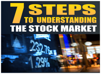
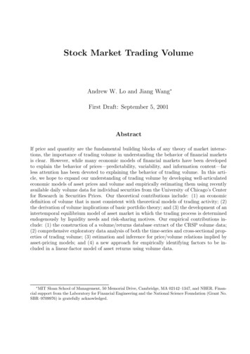
implications for the measurement and behavior of volume (see, for example, Atkins and Dyl(1997)), and this should be investigated separately.Throughout our empirical analysis, we report turnover and returns in units of percentper week—they are not annualized.Finally, in addition to the exchange and sharecode selection criteria imposed, we alsodiscard 37 securities from our sample because of a particular type of data error in the CRSPvolume entries.104Time-Series PropertiesAlthough it is difficult to develop simple intuition for the behavior of the entire timeseries/cross-section volume dataset—a dataset containing between 1,700 and 2,200 individualsecurities per week over a sample period of 1,800 weeks—some gross characteristics of volume can be observed from value-weighted and equal-weighted turnover indexes.11 Thesecharacteristics are presented in Figure 1 and in Tables 3 and 4.Figure 1a shows that value-weighted turnover has increased dramatically since the mid1960’s, growing from less than 0.20% to over 1% per week. The volatility of value-weightedturnover also increases over this period. However, equal-weighted turnover behaves somewhat differently: Figure 1b shows that it reaches a peak of nearly 2% in 1968, then declinesuntil the 1980’s when it returns to a similar level (and goes well beyond it during October 1987). These differences between the value- and equal-weighted indexes suggest thatsmaller-capitalization companies can have high turnover.NYSE/AMEX universe contained 2,307 securities with sharecode 10, 30 securities with sharecode 11, and55 securities with sharecodes other than 10 and 11. Ordinary common shares also account for the bulk ofthe market capitalization of the NYSE and AMEX (excluding ADRs of course).10Briefly, the NYSE and AMEX typically report volume in round lots of 100 shares—“45” represents 4500shares—but on occasion volume is reported in shares and this is indicated by a “Z” flag attached to theparticular observation. This Z status is relatively infrequent, is usually valid for at least a quarter, and maychange over the life of the security. In some instances, we have discovered daily share volume increasing by afactor of 100, only to decrease by a factor of 100 at a later date. While such dramatic shifts in volume is notaltogether impossible, a more plausible explanation—one that we have verified by hand in a few cases—isthat the Z flag was inadvertently omitted when in fact the Z status was in force. See Lim et al. (1998) forfurther details.11These indexes are constructed from weekly individual security turnover, where the value-weighted indexis re-weighted each week. Value-weighted and equal-weighted return indexes are also constructed in a similarfashion. Note that these return indexes do not correspond exactly to the time-aggregated CRSP valueweighted and equal-weighted return indexes because we have restricted our universe of securities to ordinarycommon shares. However, some simple statistical comparisons show that our return indexes and the CRSPreturn indexes have very similar time series properties.11

Since turnover is, by definition, an asymmetric measure of trading activity—it cannotbe negative—its empirical distribution is naturally skewed. Taking natural logarithms mayprovide more (visual) information about its behavior and this is done in Figures 1c- 1d.Although a trend is still present, there is more evidence for cyclical behavior in both indexes.Table 3 reports various summary statistics for the two indexes over the 1962–1996 sampleperiod, and Table 4 reports similar statistics for five-year subperiods. Over the entire samplethe average weekly turnover for the value-weighted and equal-weighted indexes is 0.78%and 0.91%, respectively. The standard deviation of weekly turnover for these two indexesis 0.48% and 0.37%, respectively, yielding a coefficient of variation of 0.62 for the valueweighted turnover index and 0.41 for the equal-weighted turnover index. In contrast, thecoefficients of variation for the value-weighted and equal-weighted returns indexes are 8.52and 6.91, respectively. Turnover is not nearly so variable as returns, relative to their means.12

Value-Weighted Turnover IndexEqual-Weighted Turnover Index44.32Weekly Turnover [%]. . . . . . . . . . . . . . . . . . . . . . . . . . . . . . . . . . . . . . . . . . . . . . . . . . . . . . . . . . . . . . . . . . . . . . . . . . . . . . . . . . . . . . . . . . . . . . . . . . . . . . . . . . . . . . . . . . . . . . . . . . . . . . . . . . . . . . . . . . . . . . . . . . . . . . . . . . . . . . .

the time-series and cross-sectional properties of turnover indexes, individual turnover, and portfolio turnover. Turnover indexes exhibit a clear time trend from 1962 to 1996, beginning at less than 0.5% in 1962, reaching a high of 4% in October 1987, and d