Transcription
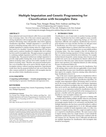
Paper 2081-2015Multiple Imputation Using the Fully Conditional Specification Method: A Comparison ofSAS , Stata, IVEware, and RPatricia A. Berglund, University of Michigan-Institute for Social ResearchABSTRACTThis presentation emphasizes use of SAS 9.4 to perform multiple imputation of missing data using thePROC MI Fully Conditional Specification (FCS) method with subsequent analysis using PROCSURVEYLOGISTIC and PROC MIANALYZE. The data set used is based on a complex sample design.Therefore, the examples correctly incorporate the complex sample features and weights. Thedemonstration is then repeated in Stata, IVEware, and R for a comparison of major software applicationsthat are capable of multiple imputation using FCS or equivalent methods and subsequent analysis ofimputed data sets based on a complex sample design.INTRODUCTIONPaper 2081-2015 presents a detailed example of multiple imputation of missing data from a complexsample design with the Fully Conditional Specification (FCS) method of PROC MI with subsequentanalysis using PROC SURVEYLOGISTIC and PROC MIANALYZE. The application is then repeatedusing Stata, IVEware, and R with an equivalent imputation method while also accounting for the complexsample design features. The application replications enable a direct comparison of results from eachsoftware tool.Analysts will gain knowledge and practical guidance for correctly implementing the three step multipleimputation process using data derived from a complex sample design data set. A general overview of themultiple imputation process is included but it is assumed that the analyst has a basic understanding of theMI process and analysis of complex sample design data.MULTIPLE IMPUTATION OF MISSING DATAMultiple Imputation is a robust and flexible option for handling missing data. MI is implemented followinga framework for estimation and inference based upon a three step process: 1) formulation of theimputation model and imputation of missing data using PROC MI with a selected method, 2) analysis ofcomplete data sets using standard SAS procedures (that assume the data are identically andindependently distributed or from a simple random sample) or SURVEY procedures for analysis of datafrom a complex sample design, and 3) analysis of the output from the two previous steps using PROCMIANALYZE (Berglund and Heeringa, 2014). A key assumption made in the MI and MIANALYZEprocedures is that the missing data are missing at random (MAR) or in other words, the probability that anobservation is missing depends on observed Y but not missing Y, (Rubin, 1987).The featured application implements the PROC MI FCS method for imputation of missing data in Step 1,use of PROC SURVEYLOGISTIC to perform design-based logistic regression in Step 2, and PROCMIANALYZE to combine results from previous steps in Step 3.THE FULLY CONDITIONAL SPECIFICATION (FCS) METHODThe Fully Conditional Specification (FCS) method is widely used for imputation of missing data for largemixed sets of continuous, nominal, ordinal, count and semi-continuous variables. The FCS method isalso labeled the sequential regression algorithm (Raghunathan, et al. , 2001) in IVEware or the “chainedequations” approach (van Buuren et al., 1999; Royston, 2005; Carlin, et al., 2008) in Stata and R.Broadly described, each of these algorithms is based on an iterative algorithm. Each iteration (t 1, ,T)of the algorithm moves one-by-one through the sequence of variables in the imputation model, e.g.Y {Y1,Y2,Y3,Y4,Y5} as illustrated in Figure 1.1
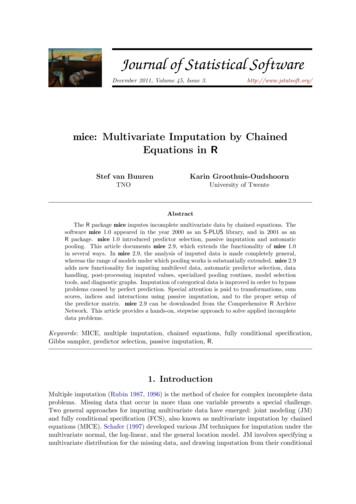
Figure 1. Arbitrary Multivariate Missing Data PatternAt each iteration and for each variable, there is a P-Step and I-Step. In the P-Step, the current (iterationt) values of the observed and imputed values for the imputation model variables are used to derive thepredictive distribution of the missing values for the target variable. To model the conditional predictivedistribution of individual Yk, PROC MI uses the same regression or discriminant function methodsavailable in PROC MI as for the monotone missing data patterns, (Berglund and Heeringa, 2014).See Figure 2 (from the SAS/STAT PROC MI documentation) for a summary of all available imputationmethods in SAS 9.4 and guidance on selection of an appropriate method.Figure 2. Table 61.5: Imputation Methods in PROC MIMULTIPLE IMPUTATION OF COMPLEX SAMPLE DESIGN DATAComplex surveys are comprised of data derived from sample designs that adjust for non-response anddiffering probabilities of selection. Complex samples differ from standard or simple random samples inthat they assume independence of observations while complex samples do not. Most SAS proceduresassume that data used is derived from a simple random sample and under-estimate variances whenanalyzing data from complex samples. Therefore, analysis of data from complex surveys should includemethods of variance estimation that account for these sample design features (Kish, 1965 and Rust,1985).The SURVEY suite of procedures (PROC SURVEYSELECT, PROC SURVEYMEANS, PROCSURVEYFREQ, PROC SURVEYREG, PROC SURVEYLOGISTIC, and PROC SURVEYPHREG) allowthe analyst to create samples and correctly analyze complex sample design data sets. However, anotherimportant consideration is how to correctly incorporate the complex sample design features and weightsinto the MI framework. Donald Rubin offered the following guidance on MI for complex samples:“Minimally, major clustering and stratification indicators and sample design weights (or estimatedpropensity scores of being in the sample) should be included in the imputation models. The possible lost2
precision when including unimportant predictors is usually a small price to pay for the general validity ofthe resultant multiply imputed data base”, (Rubin, 1996) .To capture the complex sample design features and weight(s) in the imputation model, a recommendedmethod is to create a categorical variable in the DATA STEP that is the combination of the stratum andcluster codes provided by the data producer. Then, use the combined strata and cluster variable alongwith the probability weight in the imputation model during MI Step 1. In Step 2, utilize the correct SASSURVEY procedure with weights and design variables, i.e. single STRATA, CLUSTER, and WEIGHTvariables to correctly analyze the imputed data sets and finally, use PROC MIANALYZE in MI Step 3 tocombine results and produce valid inferences.ANALYSIS APPLICATIONThe analysis application is a detailed example that uses PROC MI with the FCS method to imputemissing data on categorical variables with an arbitrary missing data pattern, analysis of imputed data setsusing PROC SURVEYLOGISTIC, and analysis of results from MI Steps 1 and 2 using PROCMIANALYZE. Because SAS is of primary interest, a detailed discussion of code, output and interpretationis included in this section.The application is then repeated using Stata, IVEware and R for direct comparison of results. For thereplications, the focus is on the final pooled estimates rather than detailed explanations of the full syntaxused. For more information on Stata, IVEware, or R, see their respective user manuals.APPLICATION DATA SETData from the National Comorbidity Survey-Replication, a nationally representative sample based on astratified, multi-stage area probability sample of the United States population (Kessler et al, 2004 andHeeringa, 1996) is used in the application. The NCS-R data set is based upon a complex sample designand contains variables representing the design features along with weights that adjust for non-response,differing probabilities of selection and post-stratification to a given population. See the project website athttp://www.hcp.med.harvard.edu/ncs/ for more information.VARIABLE LISTThe NCS-R data set is from the Part 2 of the survey (n 5,692) and includes a number of detailedquestions about DSM-IV disorders and related issues such as treatment and impairment.Variables used are in this application are as follows with variables with missing data highlighted in red: Sex Region Age Str Secu Finalp2wt Racecat Educat MDE Str Secu(categorical, coded 0 FEMALE 1 MALE)(categorical, coded 1 NE 2 MW 3 SOUTH 4 WEST)(continuous, age in years)(continuous, strata representing complex sample design)(categorical, cluster/PSU representing complex sample design)(continuous, final part 2 weight)(categorical, coded 1 WHITE 2 HISPANIC 3 BLACK 4 OTHER)(categorical, coded 1 0-11 YRS 2 12 YRS 3 13-15 YRS 4 16 YRS, some missing data)(categorical, coded 1 YES major depressive episode 0 NO MDE, some missing data)(categorical, combined Str and Secu variable)EXAMINATION OF MISSING DATAPrior to multiple imputation of missing data, an important preliminary step is to examine the data set fortypes of variables (continuous, categorical, count, etc.) that have missing data and the extent and patternof missing data. Patterns of missing data can be broadly categorized as arbitrary, monotone, ormatrix/file-matching, (see Figures 3-5 for graphic representations). Typically, identification of the missingdata pattern helps drive the choice of imputation method and number of imputed data sets created during3
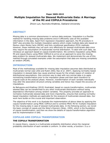
MI Step 1. For more on the question of how many imputed data sets to create, see Table 61.7 of thePROC MI documentation.Figure 3. Arbitrary Missing DataFigure 4. Monotone Missing DataFigure 5. File-Matching or Matrix Missing DataAPPLICATION USING SAS 9.4MI STEP 0 - EXPLORE MISSING DATAThe initial step, here called MI Step 0, explores the characteristics of missing data through use of PROCMI without imputation (NIMPUTE 0). PROC MI produces a Missing Data Pattern grid by default. TheSAS code below reads in a temporary data set called NCSR2 1 and creates output in Figure 6 below:proc mi nimpute 0 data ncsr2 1;run;4
Figure 6. Missing Data Patterns, NCS-R Data SetBased on Figure 6, the Model Information table contains basic information about the default imputationmethod used had there been an imputation (MCMC) along with other information related to the imputationprocess. Given that no imputation was actually performed, this information is not relevant to the processat this point.The Missing Data Patterns table reveals an arbitrary missing data pattern with two variables that requireimputation of missing data, EDUCAT and MDE. Both are classification variables (ordinal and binary,respectively) and even with re-ordering of the variables in the VAR statement, the missing data patternwould still be arbitrary. There are three distinct groups in the data set: 1. those with fully observed on allvariables (92.97% of the 5,692 observations), 2. those missing on just Major Depressive Episode (MDE,2.90%) and 3. those missing on only education in categories (EDUCAT, 4.13%). There are also twoimputation flag variables constructed in the DATA STEP (code not shown here), MDE IMP andEDUCAT IMP. These flag variables are set equal to 1 for observations that are imputed and 0 otherwise.MULTIPLE IMPUTATION STEP 1 - IMPUTE MISSING DATAMI Step 1 uses PROC MI to impute missing data. The FCS imputation method is selected because iteasily handles arbitrary missing data patterns with continuous or classification variables that needimputation.The following code uses PROC MI to create a default 5 imputed data sets (NIMPUTE 5) using a SEEDvalue (SEED 876) and creates a temporary output data set containing the (OUT OUTFCS). In addition,the CLASS statement declares sex, region, race, education, MDE, and the combined strata and clustervariable as classification variables (CLASS SEX REGION RACECAT EDUCAT MDE STR SECU). TheFCS LOGISTIC statement requests the FCS logistic regression method with 40 burn-in iterations(NBITER 40) and model details (DETAILS) for each of the five imputation models used to impute MDE.Note that both variables to be imputed are binary (MDE) or ordinal (EDUCAT) and the LOGISTIC methodis appropriate for both.The VAR statement lists the variables to be used in the imputation models and omits the imputation flagvariables as they do not have any scientific meaning in the imputation model. The final Part 2 NCS-Rweight (FINALP2WT) and the combined strata and cluster variable (STR SECU) are used as imputationmodel covariates to represent the complex sample design features and probability weight. Other modelcovariates include gender, US region, age at interview, race, and the imputed MDE (after MDE is imputedduring the process). By default, PROC MI imputes the variables following the order in the VAR statementtherefore, fully observed variables are listed first (SEX REGION AGE RACECAT STR SECUFINALP2WT) followed by those with the least to the most missing data (MDE EDUCAT).5
The output data set (OUTFCS) contains five imputed data sets stored in a "long" format along with a SASgenerated variable called IMPUTATION with values of 1-5 to identify each imputed data set. Therefore,the output data set contains 5*5,692 28,460 observations:proc mi data ncsr2 1 seed 876 nimpute 5 out outfcs;class sex region racecat educat mde str secu;fcs nbiter 40 logistic (mde/details) logistic (educat);var sex region age racecat str secu finalp2wt mde educat;run;Figure 7. Selected Output from the PROC MI FCS IMPUTATIONFrom Figure 7, the Model Information Table lists the FCS Method, Number of Burn-In Iterations andrandom number generator specified in the code. The FCS Model Specification lists the variables thatrequire imputation along with Regression and Discriminant Function methods with associated variablesfor each method. Since the variables listed under the Regression and Discriminant Function methods arefully observed, the default methods are listed but no data is actually imputed for these variables.6
The Missing Data Patterns grid displays the extent of missing data by group along with Group Means forjust the continuous variables used in the imputation. Finally, the Logistic Models for FCS Method table(partial output presented) details the parameter estimates for each of five imputed data sets and for eachlevel of the Effects. This level of detail is produced by the DETAILS option in the FCS statement and canbe used as a diagnostic tool to evaluate the individual imputations. This output shows stable estimatesacross all 5 imputations of MDE for the effects sex, region, age, and race effects.The code below illustrates use of PROC FREQ to produce unweighted cross-tabulations of observedMDE by imputed MDE (MDE*MDE IMP), for each of the 5 imputed data sets. This type of informaldiagnostic check permits evaluation of the observed v. imputed variable distributions with the aim ofidentifying possible problems in the imputation:proc freq data outfcs;tables imputation *mde*mde imp / missing;run;Figure 8. Cross-Tabulations of Observed MDE and Imputed MDE by Imputation, For Data Sets 1 and 2 OnlyThe cross-tabulations in Figure 8 reveal how the values of imputed MDE differ across the imputed datasets (just results from imputations 1 and 2 are shown here). These slight differences reflect the expectedrandom variability of the imputation process and present no evidence of problems in the imputation. For7
example, for IMPUTATION 1, 67.27% of the respondents are imputed to MDE 0 and 32.73% areimputed to MDE 1. In comparison, the observed percentages are 68.45% (MDE 0) and 31.55%(MDE 1). The second imputed data set ( IMPUTATION 2) shows similar differences between observedand imputed percentages. Other PROC MI diagnostic tools such as TRACE and AUTOCORRELATIONplots are available for continuous variables, see the documentation for details and examples.MULTIPLE IMPUTATION STEP 2 - ANALYZE IMPUTED DATA SETS USING PROCSURVEYLOGISTICWith five imputed data sets produced in MI Step 1, MI Step 2 consists of analysis of the completed datasets using the SURVEY procedure of choice. The planned analysis for this example is a design-basedlogistic regression predicting the probability of having a diagnosis of lifetime Major Depressive Episodewith gender, education, and US region covariates. Note that all of the variables to be used in the analysisplus additional covariates including the weight and complex sample design variables were included in theimputation models. In general, the imputation model should include, at the minimum, all analysis modelvariables plus additional meaningful covariates to enhance the imputations.The code below reads the five imputed data sets stored in the OUTFCS data set (DATA OUTFCS), theSTRATA, CLUSTER, and WEIGHT statements represent the complex sample design and weights, and aCLASS statement is used with a REF option to declare classification variables and custom referencegroups along with the PARAM REF option to request reference group parameterization. Each designbased logistic regression is run separately within each imputed data set due to BY statement (BYIMPUTATION ) and an output data set of parameter estimates and standard errors is created by ODSOUTPUT PARAMETERESTIMATES OUTPARMS statement.The PRINT procedure produces a listing report of the output data set from PROC SURVEYLOGISTIC.This data set will serve as input for PROC MIANALYZE in MI Step 3 and should contain, at a minimum,parameter estimates and variance information for univariate inference in MIANALYZE:proc surveylogistic data outfcs;strata str; cluster secu; weight finalp2wt;class sex (ref '0') educat (ref '1') region (ref '1') / param ref;model mde (event '1') sex educat region;by imputation ;ods output parameterestimates outparms;run;proc print data outparms;run;8
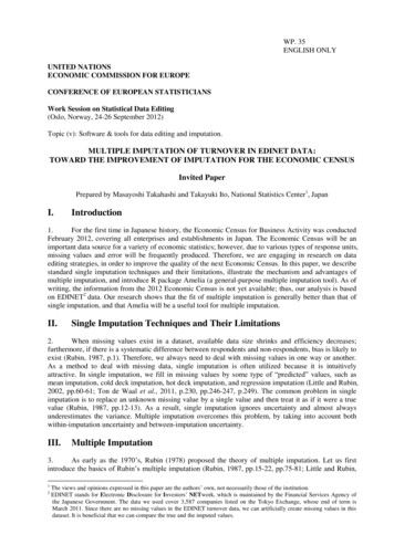
Figure 9. Partial Listing of the OUTPARMS Data Set from PROC SURVEYLOGISTIC, Imputation Data Sets 1and 2Figure 9 displays records from the OUTPARMS data set and includes a variable called IMPUTATIONwith values of 1-5, Variable with the names of the model effects, CLASSVAL0 with the Class variablelevel, the degrees of freedom, estimated parameters and standard errors, and Wald Chi-Square valuesand associated p values.MULTIPLE IMPUTATION STEP 3 - COMBINE RESULTS FROM MI STEPS 1 AND 2 AND GENERATEVALID INFERENCES USING PROC MIANALYZEThe third step of the MI process combines results from Steps 1 and 2 and generates valid inferencesusing PROC MIANALYZE. As a reminder, the output data set from Step 2 contains estimated weightedparameter estimates from the logistic regression predicting lifetime MDE with design-based standarderrors from PROC SURVEYLOGISTIC. There are five sets of parameter estimates and standard errorsthat are combined by PROC MIANALYZE to reflect the variability of the imputation process along with thecomplex sample design features.The following syntax executes PROC MIANALYZE and performs univariate inference. The PROCstatement declares the OUTPARMS data set as a PARMS type of data set with classification variablesread in with the CLASSVAL option (PARMS (CLASSVAR CLASSVAL) OUTPARMS). This optioninstructs SAS to read each CLASS variable's levels from the variable CLASSVAL0. The CLASSstatement sets SEX, EDUCAT, and REGION as classification variables and omits the category specifiedin the SURVEYLOGISTIC code, the lowest category for each variable in the CLASS statement in thisexample. The MODELEFFECTS statement lists the model covariates, beginning with the intercept, in theorder established in the previous step. Though this examples produces only univariate inferences,multivariate inference is possible in PROC MIANALYZE, see the SAS/STAT MIANALYZE documentationfor details and examples:proc mianalyze parms (classvar classval) outparms;class sex educat region;modeleffects intercept sex educat region;run;9
Figure 10. Model Information, Variance Information and Multiple Imputation Logistic Regression ParameterEstimates for MDE: SAS Results from PROC MIANALYZEFigure 10 includes selected tables from PROC MIANALYZE including Model Information, VarianceInformation, and Parameter Estimates. The Model Information lists the input OUTPARMS data set with 5imputations.The Variance Information table includes the between, within, and total variances for each parameter inthe model. The table details the relative increase in variance due to missing data (range from 0.003 to0.12) and Fraction Missing Information (range from 0.004 to 0.12) which reflects the impact of missingdata among the variables used in the regression model. Based on five imputed data sets, RelativeEfficiency is close to 1.0 for all effects, suggesting that five imputations are sufficient.The Parameter Estimates represent averaged estimates with standard errors that are adjusted for boththe complex sample design and the variability introduced by multiple imputation. Therefore, 95%confidence limits and t tests are based on the fully corrected standard errors.These results suggest that men are significantly less likely than women to have an MDE diagnosis, thosein higher education groups are more likely than the lowest educational group (0-11 years of education) tohave MDE but only the group with 13-15 years of education is significant at the 0.05 alpha level. Theresults for US regions indicate that those in Midwest and West are more likely to have MDE as comparedto those in the Northeast region while those in the South region are less likely than the Northeast region10
to have MDE. None of the individual region predictors are significant and all results are interpreted whileholding all other predictors in the model constant.APPLICATION REPLICATIONS USING IVEWARE, STATA AND R SOFTWAREIVEWAREIVEware (Imputation and Variance Estimation Software) is a software designed to perform multipleimputation of missing data and subsequent analysis of data derived from complex sample designs. Ituses the sequential regression method (also known as FCS or chained equations) to perform multipleimputation along with the Jackknife Repeated Replication (JRR) method for complex sample varianceestimation.In this demonstration, IVEware is used as a SAS-callable tool though it is also possible to run thesoftware as a standalone version, see iveware.org for more information and downloads. The softwareperforms imputation with the %IMPUTE macro and regression analysis with correct variance estimationwith the %REGRESS macro and descriptive analysis with the %DESCRIBE macro. The macros are runfrom the regular (not enhanced) SAS program editor and SAS programmers with a basic understandingof how to invoke macros can execute the IVEware program without the need to learn a new language.The following syntax reads in the SAS data set named NCSR2 1 and performs preliminary recodes in theDATA STEP prior to multiple imputation. The %IMPUTE macro imputes missing data using thesequential regression method and creates 5 multiples or imputed data sets. This macro call uses anumber of additional statements to control the imputation. For example, the default variable type is set toCONTINUOUS while classification variables are declared as CATEGORICAL and the remainingvariables in the data set are declared as TRANSFER, meaning these variables are retained but not usedin the imputation models. A SEED value is used to ensure future replication of the results andMULTIPLES is set to 5 to produce five imputed data sets:data app4;set ncsr2 1;* Recode the dependent variable to make highest category (no) the omitted;if mde 0 then mde r 2; else if mde 1 then mde r 1; else mde r .;run ;%impute (name app4, setup new, dir . );datain app4;dataout app4 imp;default continuous;categorical sex region racecat educat mde r str secu;transfer sampleid mde imp educat imp str secu mde;multiples 5;seed 876;run;After imputation, the %PUTDATA macro outputs five temporary SAS data sets (IMP1-IMP5) to be usedas input to the %REGRESS macro. %REGRESS performs design-based logistic regression with theJRR variance estimation method while the LINK LOGISTIC statement requests a logistic regression usingthe outcome variable MDE R. This recoded variable predicts the probability of having MDE (coded as 1)while no MDE (coded as 2) serves as the omitted category. Since IVEware omits the highest category ofany categorical variable, the reference categories differ from SAS, Stata, and R. An alternative is to useindicator variables representing each level of the categorical variables and omit the lowest category tomatch the other programs (not shown here).Use of the complex sample design variables and weight with the five imputed input data sets produceregression results that incorporate the imputation variability and complex sample design features:11
* use %putdata to produce 5 separate data sets for correct MI estimation;%putdata(name app4,dir ., mult 1,dataout imp1 );%putdata(name app4,dir ., mult 2,dataout imp2 );%putdata(name app4,dir ., mult 3,dataout imp3 );%putdata(name app4,dir ., mult 4,dataout imp4 );%putdata(name app4,dir ., mult 5,dataout imp5 );%regress (name app4 2, setup new, dir . );datain imp1 imp2 imp3 imp4 imp5;stratum str;cluster secu;weight finalp2wt;categorical sex educat region;predictor sex educat region;dependent mde r;link logistic;run ;Figure 11. Multiple Imputation Logistic Regression of MDE: Results From IVEwareFigure 11 includes parameter estimates with JRR based variance estimates, Wald tests, Odds Ratios with95% Confidence Limits, Design Effects, SRS estimates, and the percentage difference between the SRSand design-based Estimates. The variances are adjusted for the variability due to the MI process as well12
as the complex sample design features and weight. Interpretation of the results is included in a latersection where the results from all four software packages are contrasted.STATAThe next replication uses Stata (v13.1) to impute missing data and analyze imputed data sets while takingthe complex sample design features and weight into account. Stata offers a number of multipleimputation and survey commands within the mi and svy suite of commands, see the Stata documentationfor details.The command syntax below reads the input data set, sets up the multiple imputation by registeringimputed and regular (not imputed) variables, imputes missing data using the "chained equations" method,sets the survey variables and then performs an MI and design-based analysis using the mi estimate:svy:logit command:* read data set into memoryuse "ncsr2 v12.dta", clear* set up mi data and register variablesmi set mlongmi register imputed mde educatmi register regular sex region racecat age finalp2wt str secu str secu* impute missing data using chained logit, ologit commandsmi impute chained (logit) mde (ologit) educat i.sex i.region ///i.racecat age finalp2wt i.str secu , add(5) rseed(2012)* set survey variables within the mi suite of commandsmi svyset secu [pweight finalp2wt], strata(str)* run mi estimate: svy logit regressionmi estimate: svy: logit mde i.sex i.region i.educatMultiple-imputation estimatesSurvey: Logistic regressionNumber of strata 42Number of PSUs 84DF adjustment:Model F test:Within VCE type:Small sampleEqual FMILinearized13ImputationsNumber of obsPopulation size 5 5692 5692.0005Average RVILargest FMIComplete DFDF:minavgmaxF(7,39.7)Prob F 0.04640.09334234.4638.4339.7916.020.0000
---------------------------mde Coef.Std. Err.tP t [95% Conf. Interval]------------- -------------1.sex -.5111926.0638813-8.000.000-.6403719-.3820132 region 2 .0065904.14080850.050.963-.2783006.29148143 -.1669361.1330025-1.260.217-.4358414.10196924 .039644.13198370.300.765-.2271491.3064372 educat 2 .094891.10744640.880.383-.1228383.31262043 .2324122.11240722.070.046.004085.46073934 .1770819.11144831.590.120-.0482573.4024212 cons e 12. Multiple Imputation Logistic Regression of MDE: Results From StataFigure 12 includes information about the number of imputations contained in the multiply imputed data set(5), variance information such as Average RVI (Relative Variance Increase) and Largest FMI (FractionMissing Information), Degrees of Freedom (complete and Small Sample adjusted), and an F test for themodel. In addition, parameter estimates, standard errors, t tests and p values, and 95% confidenceintervals that account for the MI process and the complex sample design are presented. As with IVEwareand R, interpretation of results is done in the last section of this paper.RThe final replication uses R v3.0.1 with the mice, mitools, foreign, and survey packages to impute missingdata using chained equations and analyze imputed data sets with mitools commands and the svyglmcommand for design-based logistic regression that also accounts for the multiple imputation variability.The following code loads the needed R packages, reads in a Stata format data set and translates for usein R, creates factor variables for use in the multiple imputation and subsequent analyses, imputes missingdata using the mice (multiple imputation by chained equations) command, and converts the output MIdata to a format acceptable for use with the mitools package. Then, the syntax sets the complex sampledesign variables and weight and executes the svyglm command with the correct family option to performa multiple imputation, design-based logistic regression while using the five imputed data sets with theMIcombine command:# load packages using library commandlibrary(foreign)library(mi)library(mice)# read Stata format data set into Ra - read.dta("C:/ncsr2 v12.dta" )summary(a)# create factor variablesa sex - factor(a sex)a educat - factor (a educat)a region - factor(a region)a str secu - factor(a str secu)# obtain information about missing data14
inf -mi.info(a)# print info about missing datainf# use mice to impute and poollibrary(mice)imp - mice(a,n.imp 5,seed 1934)summary(imp)# convert mids to data useable for work in mitoolslibrary(mitools)mydata - imputationList(lapply(1:5, complete, x imp))summary(mydata)# set surve
Multiple Imputation is a robust and flexible option for handling missing data. MI is implemented following a framework for estimation and inference based upon a three step process: 1) formulation of the imputation model and imputation of missing data using PROC MI with a selected method, 2) analysis of