Transcription
Paper 3605-2019Multiple Imputation for Skewed Multivariate Data: A Marriageof the MI and COPULA ProceduresZhixin Lun, Ravindra Khattree, Oakland UniversityABSTRACTMissing data is a common phenomenon in various data analyses. Imputation is a flexiblemethod for handling missing-data problems since it efficiently uses all the availableinformation in the data. Apart from regression imputation approach, the MI procedure inSAS also provides the multiple imputation options which create multiple data sets based onMarkov chain Monte Carlo (MCMC) and fully conditional specification (FCS) methods.However, these methods may not work very effectively for skewed multivariate data sincethey require the assumption of multivariate normal distribution. To deal with such data, weintroduce an approach based on copula transformation. We combine imputation using PROCMI and copula theory using PROC COPULA to arrive at an approach to solve the missingdata problem for skewed multivariate data. We implement and demonstrate the use of thismethod through simulated examples under the assumption that data are missing completelyat random (MCAR).INTRODUCTIONMost of the methodology available for missing data imputation assumes data distributed asmultivariate normal (see Little and Rubin 2002, Rao et al. 2007). Applying normality-basedimputation in skewed data may cause practical issues for the simple reason of violation ofdistributional assumptions. One common way to deal with non-normal data is to applynormalizing transformation prior to the imputation phase and then back-transform tooriginal scale at the analysis phase. However, transformation of each variable individuallymay alter the association structure among variables and hence may impact the accuracy ofimputations.As Bahuguna and Khattree (2019) illustrated, based on copula transformation, multivariateskewed data can be transformed to any other multivariate distribution without losingdependence information among random variables. This property provides an approach tonormalize multivariate skewed data and more importantly, ensures that existing normalitybased imputation methods are applicable for the analysis of multivariate skewed data. Ourwork here builds on this crucial and important observation.The objective of this work is to illustrate the implementation of above ideas by applying thecopula transformation using PROC COPULA and to combine PROC MI for multiple imputationfor the missing data in case of skewed multivariate data. In the following section, we revisitthe basic concept of copula and the Sklar's theorem (Sklar, 1959), which is the foundationof copula transformation, and then we show the details of copula transformation algorithmand its implementation in SAS.COPULAS AND COPULA TRANSFORMATIONTHE COPULA TRANSFORMATIONIn copula theory, copula is a multivariate probability distribution where the marginalprobability distribution of each variable is uniform. In other words, a function 𝐶 is a 𝑑-1
dimensional copula if there is a random vector 𝑈 (𝑈1 , 𝑈2 , , 𝑈𝑑 )′ , such that for 𝑖 1,2, , 𝑑,𝑈𝑖 Uniform (0,1), and𝐶(𝑢1 , 𝑢2 , , 𝑢𝑑 ) 𝑃[𝑈1 𝑢1 , 𝑈2 𝑢2 , , 𝑈𝑑 𝑢𝑑 ].The most important theorem in copula theory is the Sklar's theorem (Sklar, 1959), whichstates that a function F: Rd [0,1] is the distribution function of a random vector 𝑋 (𝑋1 , 𝑋2 , , 𝑋𝑑 )′ if and only if there is a copula 𝐶 from [0,1]𝑑 to [0,1] and 𝑑 univariate distributionfunctions 𝐹1 , 𝐹2 , , 𝐹𝑑 such that𝐶(𝐹1 (𝑥1 ), 𝐹2 (𝑥2 ), , 𝐹𝑑 (𝑥𝑑 )) 𝐹(𝑥1 , 𝑥2 , , 𝑥𝑑 ).This theorem indirectly implies that two different continuous multivariate distributions canbe transformed to each other via the same copula. Specifically, consider two differentcontinuous multivariate cumulative distributions denoted by 𝐹( ) and 𝐺( ) and assume thatthey have a common copula. Then the transformation is shown as follows from Sklar'stheorem,𝑭(𝒙𝟏 , 𝒙𝟐 , , 𝒙𝒅 ) 𝑪(𝑭𝟏 (𝒙𝟏 ), 𝑭𝟐 (𝒙𝟐 ), , 𝑭𝒅 (𝒙𝒅 )) 𝑪(𝒖𝟏 , 𝒖𝟐 , , 𝒖𝒅 ) 𝑪(𝑮𝟏 (𝒚𝟏 ), 𝑮𝟐 (𝒚𝟐 ), , 𝑮𝒅 (𝒚𝒅 )) 𝑮(𝒚𝟏 , 𝒚𝟐 , , 𝒚𝒅 ),(𝟏)where 𝐹𝑖 ( ) and 𝐺𝑖 ( ) are the corresponding marginal cumulative distribution functions arisingout of 𝐹( ) and 𝐺( ), respectively. Thus, a set of data on (𝑥1 , , 𝑥𝑑 ) can be transformed as(𝑦1 , , 𝑦𝑑 ) and vice versa via dependent uniform data (𝑢1 , 𝑢2 , , 𝑢𝑑 )′ created in between.In this study, since our purpose is to normalize multivariate variables, we assume that thecommon copula is a Gaussian copula Φμ,Σ ( ), that is,𝐶Σ (𝑢1 , , 𝑢𝑑 ) Φμ,Σ (Φ 1 (𝑢1 ), , Φ 1 (𝑢𝑑 )),where Φμ,Σ ( ) is the cumulative distribution of multivariate normal distribution with meanvector 𝜇 and covariance matrix Σ. Φ( ) is the cumulative distribution function of the standardunivariate normal and Φ 1 ( ) is its inverse function.THE ALGORITHMWe start with the missing data problem, for which missingness occurs in one variabledenoted by 𝐘 while the other variables 𝐗 i 's are fully observed. Then the missing datastructure can be divided into two blocks: (i) the complete cases denoted by (𝐘obs , 𝐗 cc ) and(ii) incomplete cases denoted by (𝐘mis , 𝐗 ic ). Let𝐘(𝐘, 𝐗) [ 𝐨𝐛𝐬𝐘𝐦𝐢𝐬𝐗 𝐜𝐜].𝐗 𝐢𝐜According to the above process of copula transformation as stated in Equation (1), weimplement the following algorithm,1. Transform the complete cases (𝐘𝐨𝐛𝐬 , 𝐗 𝐜𝐜 ) to uniformly distributed data 𝐔𝐜𝐜 (𝑈𝑌 , 𝑈𝑋1 , 𝑈𝑋2 , , 𝑈𝑋𝑘 ) using the empirical cumulative distribution function estimated fromthe data.2. For the incomplete case, transform 𝐗 𝐢𝐜 to uniformly distributed data 𝐔𝐢𝐜 (𝑈𝑋1 , 𝑈𝑋2 , , 𝑈𝑋𝑘 )using the empirical cumulative distribution function estimated from the data. There is no2
𝑈𝑌 data due to missingness.3. Combine 𝐔𝐜𝐜 and 𝐔𝐢𝐜 into 𝐔, that is𝐔 [𝐔𝑐𝑐],𝐔𝑖𝑐and convert 𝐔 to a new dataset (𝐘 , 𝐗 ) using inverse multivariate normal cumulativedistribution, corresponding to the correlation matrix from the original data. Thus,(𝐘 , 𝐗 ) [ 𝐘𝐨𝐛𝐬 𝐘𝐦𝐢𝐬𝐗 𝐜𝐜 ].𝐗 𝐢𝐜At this stage, after transforming from 𝐔 to (𝐘 , 𝐗 ), one of the imputation methods can beapplied on multivariate normally distributed (𝐘 , 𝐗 ) as in Step 4 below.4. Use one of the imputation procedures (e.g. regression, MCMC, FCS) as desired to impute all missing values of 𝐘𝐦𝐢𝐬. Multivariate normality of (𝐘 , 𝐗 ) makes this step easilyimplementable using PROC MI.5. Back-transform the filled-in data to original scale via 𝐔 according to the chosen copulafunction.It is assumed that the missingness scheme is independent of any such transformation andhence will remain the same all through the transformation.IMPLEMENTATIONWe illustrate the implementation scheme step by step following the above algorithm on asample dataset misData with four variables (𝑌, 𝑋1 , 𝑋2 , 𝑋3 ), which contains missing values in 𝑌and fully observed values in 𝑋1 , 𝑋2 , and 𝑋3 . We add an indicator column Flag into the datasetmisData such that Flag 'X' and '.' are for complete and incomplete cases, respectively.Step 1 & 2: Transform complete cases (𝐘𝑜𝑏𝑠 , 𝑿𝑐𝑐 ) and incomplete cases 𝐗 𝑖𝑐 to uniformrandom variables using PROC COPULA, respectively. We specify parameter normal in FITstatement since we use Gaussian copula. The setting marginals empirical indicates thatwe use the empirical cumulative distribution function estimated from the data. The resultingdataset unif cc star is the data set on the transformed uniform variables from completecases (𝐘𝑜𝑏𝑠 , 𝐗 𝑐𝑐 ), while unif ic star is the data set on the transformed uniform variablesfrom incomplete cases 𝐗 𝑖𝑐 .%let misVar y;%let ccVarList x1 x2 x3;proc copula data misData(where (Flag 'X'));var &misVar &ccVarList;fit normal / marginals empirical outpseudo unif cc noprint;run;proc copula data misData;var &ccVarList;fit normal / marginals empirical outpseudo unif ic noprint;run;data unif cc star;set unif cc;Flag 'X';run;3
data unif ic star(where (Flag '.'));merge unif ic misData(keep Flag);run;Step 3: Combine two datasets unif cc star and unif ic star and transform each ofuniformly distributed column data to standard normal by using quantile function.data unif u;set unif cc star unif ic star;run;data std norm;set unif u;if Flag 'X' then y quantile("Normal", y);x1 quantile("Normal", x1);x2 quantile("Normal", x2);x3 quantile("Normal", x3);run;Step 4: Apply the desired multiple imputation method on the dataset std norm. MCMCmethod is selected as an example in the code given below.proc mi data std norm nimpute 5 out mi std norm seed 1234 noprint;mcmc;var &misVar &ccVarList;run;Step 5: Note that the imputed values in above dataset mi std norm are still in standardnormal scale. The last step is to back-transform the filled-in data to original scale accordingto the copula. This process involves two steps:(a) Simulate a large number (e.g., NSIM 10,000) of observations from multivariate uniformdistribution corresponding to our copula and convert those simulated observations to thedata on variables in original data scale and to the data on variables with standard normaldistribution, respectively. This can be readily simulated by using FIT and SIMULATEstatements in PROC COPULA. The FIT statement setting must be the same as we set in Step1 & 2 since we back-transform the data according to the same copula. The output datasetsim org contains the simulated observations in original scale and sim unif consists of thesimulated observations distributed as multivariate uniform distribution. The datasetsim std norm is the converted data where each variable is distributed as standard normal.%let NSIM 10000;proc copula data misdata(where (Flag 'X'));var &misVar &ccVarList;fit normal / marginals empirical noprint;simulate /ndraws &NSIM seed 1234567out sim org outuniform sim unif;run;data sim std norm;set sim unif;sy quantile("Normal", y);sx1 quantile("Normal", x1);4
sx2 quantile("Normal", x2);sx3 quantile("Normal", x3);keep sy sx1 sx2 sx3;run;(b) Obtain the imputed values in original data scale by interpolation from above simulatedobservations in data sets sim org and sim std norm. Denote the imputed value in Step 4by 𝑦̂,̂𝑘 is sandwiched between two values 𝑠𝑦𝑡 and𝑘 which is in standard normal scale. If 𝑦𝑠𝑦𝑡 1 in dataset sim std norm, then we predict 𝑦𝑘 in its original scale by averaging, ingeneral, by interpolating values corresponding to 𝑠𝑦𝑡 and 𝑠𝑦𝑡 1 in dataset sim org. In theresulting dataset impt org scale, the variable ry with MIS 'Y' are the imputed values inoriginal scale.data sim org;set sim org;keep y;rename y ry;run;data sim std norm(keep sy);set sim std norm;run;proc sort data sim std norm; by sy; run;proc sort data sim org; by ry; run;data sim org std;merge sim std norm sim org;run;/* filter the imputed values in variable y*/data impt std norm;set mi std norm(where (Flag '.'));keep y;rename y sy;run;data impt sim comb;set impt std norm sim org std;run;proc sort data impt sim comb; by sy; run;data impt org scale;merge impt sim comb impt sim comb(keep ry firstobs 2rename (ry lead mis));lag mis lag(ry);if ry . then do;ry mean(lag mis, lead mis);MIS 'Y';end;run;5
AN ILLUSTRATION VIA SIMULATED DATA SETSCOMPLETE DATA GENERATION AND MISSINGNESS MECHANISMUsing the Iman-Conover method given by Wicklin (2013), we generate data sets from thefollowing two multivariate distributions, where marginals of components are as specified inTable 1,Group𝑋1𝑋2𝑋3𝑋41Log-normal (0, 𝜎)Pareto (1,1)Normal (0,1)Uniform (0,1)2Log-normal (0, 𝜎)Normal (0,1)Exponential (1)Uniform (0,1)Table 1. Marginal distributions of simulated data setswhere 𝜎 was set as 1.0, 2.0 and 3.0. In each case, the following correlation structure wasused,1ρCorr [ρρρ1ρρρρ1ρρρ]ρ1where ρ was set as 0.9.Missing values are assumed to be missing completely at random (MCAR).EVALUATION OF OUR IMPUTATION METHODWe select 𝑋1 as the variate with missing values. The sample size is taken as 100 and thenumber of missing cases as 5. To evaluate the quality of imputation, we simulate eachscenario NSIM 1,000 times and use 𝑘 imputation(s). Then we compute the mean of thesum of squared residuals byNSIM𝑘521impt(𝑚)𝑡𝑟𝑢𝑒MSSR (𝑋1𝑖 𝑋1𝑖) ,NSIM𝑚 1 𝑖 1impt(𝑚)𝑡𝑟𝑢𝑒where 𝑋1𝑖is the 𝑚-th imputed value for the 𝑖-th missing value 𝑋1𝑖 and 𝑋1𝑖is the trueobserved value of 𝑋1𝑖 .MULTIPLE IMPUTATION METHODSWe select FCS regression (Van Buuren 2007) and MCMC (Schafer 1997) multiple imputationmethods for multiple imputation. The general idea of FCS regression is to generate 𝑘 sets ofpredicted values based on regression model, which involves filled-in phase and imputationphrase. MCMC method is used to generate 𝑘 sets of predicted values according to theposterior distributions in Bayesian inference. Both methods require the assumption that thedata are from a multivariate normal distribution. In our illustration, we choose 𝑘 5.SIMULATION RESULTTable 2 and Table 3 give sample summaries using FCS and MCMC methods for original andcopula-transformed data. The column Ratio (O/C) is the ratio of the MSSR values of aboveto respective data. The larger Ratio (O/C) indicates the better performance of copula6
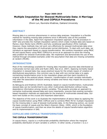
transformation. The column %SSR (O C) is the percent of times our approach results insmaller sum of squared residuals. Accordingly, the larger percentage value indicatessuperior performance of our transformation approach. The following results show that ourapproach performs substantially better than the case when multivariate normality of thedata was blindly assumed. A more detailed extensive simulation work, not reported heredue to lack of space, confirms to the above observations.MethodMSSR𝝈Original(Assumed medRatio(O/C)(O 9%3.067,349,495.8513,494,377.604.9985.5%Table 2 Comparison between original data and copula-transformed data usingmultiple imputation (𝒌 𝟓) for Group 1 with correlation choosing 𝝆 𝟎. 𝟗MethodMSSR𝝈Original(Assumed medRatio(O/C)(O 235,290.8429,549,312.571.5085.5%Table 3 Comparison between original data and copula-transformed data usingmultiple imputation (𝒌 𝟓) for Group 2 with correlation choosing 𝝆 𝟎. 𝟗CONCLUSIONWe have introduced a very powerful approach based on copula transformation to impute themissing values for general skewed multivariate data. We provide the algorithm and itsimplementation for one-variate missing pattern. Algorithm can be readily modified for 𝑘variate (𝑘 1) missing patterns. In view of ready accessibility of MI and COPULAprocedures, this approach has a very wide scope for practical applications. A complete7
program combining all the procedures pieces is given as the supplementary material. Anexecution of our program results in imputed values (column rx1 in bold) shown in Table 4for five missing values.Obs Imputationsx1sx2sx3sx4Flag Srrx1MIS11-0.71624 -0.88485 -0.62092 -0.39469.10.61905Y21-1.15206 -1.28721 -1.48097 -2.33008.20.42109Y31-0.41595 -0.71397 -0.11191 -0.47658.30.92597Y410.374300.561790.65130 Y0.16202Table 4 The first five output (the imputed values are in column rx1 in bold) ofexecution of sample code in supplementary materialREFERENCESBahuguna, M. and Khattree, R. 2019. “A Generic All Purpose Transformation for MultivariateModeling through Copulas.” To appear in International Journal of Data Science andAnalytics.Little, R.J.A. and Rubin, D.B. 2002. Statistical Analysis with Missing Data. 2nd Edition.Hoboken, NJ: John Wiley & Sons.Rao, C.R., Toutenburg, H., Shalabh, Heumann, C. 2007. Linear Models and Generalizations,Least Squares and Alternatives. 3rd Extended Edition. New York, NY: Springer.SAS Institute 2014. SAS/ETS 13.2 User's Guide The COPULA Procedure. Cary, NC: SASInstitute Inc.SAS Institute 2017. SAS/STAT 14.3 User's Guide The MI Procedure. Cary, NC: SAS InstituteInc.Sklar, A. 1959. "Distribution Functions of n Dimensions and Margins," Publications of theInstitute of Statistics of the University of Paris, 8: 229-231.Schafer, J.L. 1997. Analysis of Incomplete Multivariate Data. London: Chapman & Hall.Van Buuren, S. 2007. “Multiple Imputation of Discrete and Continuous Data by FullyConditional Specification.” Statistical Methods in Medical Research, 16:219-242.Wicklin, R. 2013. Simulating Data with SAS. Cary, NC: SAS Institute Inc.CONTACT INFORMATIONYour comments and questions are valued and encouraged. Contact the author at:Zhixin Lun, PhD StudentDepartment of Mathematics and Statistics, Oakland a Khattree, Professor/Co-directorDepartment of Mathematics and Statistics/Center for Data Science and Big DataAnalytics, Oakland Universitykhattree@oakland.edu8
SAS and all other SAS Institute Inc. product or service names are registered trademarks ortrademarks of SAS Institute Inc. in the USA and other countries. indicates USAregistration.Other brand and product names are trademarks of their respective companies.9
Multiple Imputation for Skewed Multivariate Data: A Marriage of the MI and COPULA Procedures Zhixin Lun, Ravindra Khattree, Oakland University ABSTRACT Missing data is a common phenomenon in various data analyses. Imputation is a flexible method for handling missing-data problems since it efficiently uses all the available information in the data.