Transcription
Paper 1738-2018Using SAS for Multiple Imputation and Analysis of Longitudinal DataPatricia A. Berglund, Institute for Social Research-University of MichiganABSTRACT“Using SAS for Multiple Imputation and Analysis of Data” presents use of SAS to address missing dataissues and analysis of longitudinal data. Appropriate multiple imputation and analytic methods areevaluated and demonstrated through an analysis application using longitudinal survey data with missingdata issues.The analysis application demonstrates detailed data management steps required for imputation andanalysis, multiple imputation of missing data values, subsequent analysis of imputed data, and finally,interpretation of longitudinal data analysis results. Key SAS tools including data step operations toproduce needed data structures and use of PROC MI, PROC MIANALYZE, PROC MIXED, and PROCSGPLOT are highlighted.INTRODUCTIONThis paper presents a discussion of missing data issues, evaluation of multiple imputation and analysismethods appropriate for longitudinal data, and a detailed analysis application using SAS tools.The application uses data from the Panel Study of Income Dynamics (PSID). This rich, longitudinalsurvey includes information on the family head ’s income for many years and presents an opportunity toemploy descriptive methods and regression techniques, once missing data problems are addressed.SAS DATA STEP tools for data restructuring and use of PROC MI, PROC MIANALYZE, PROC SGPLOTand PROC MIXED are highlighted in the application.The content of paper 1738 is useful to those working with longitundinal data with missing data problemsand the need for an integrated process for multiple imputation and analysis of completed longitudinal datasets. Skills taught include how to use SAS to address missing data in longitudinal data sets, analyzecompleted data sets using appropriate descriptive and regression techniques, and combine results whileaccounting for both imputation variability and if needed, complex sample design features for correctvariance estimation.SECTION 1-OVERVIEW OF MISSING DATA AND MULTIPLE IMPUTATIONMISSING DATA IN LONGITUDINAL DATA SETSMissing data is especially common in longitudinal data sets. Reasons for the missingness might berespondent attrition, survey structure where some questions are asked only of a sub-set of respondents,file-matching issues where some variables are not included in all data sets used in a merge process, andrefusal to answer sensitive questions such as income, illegal behaviors, or certain health conditions.Missing data is generally categorized as Missing at Random (MAR), Missing Completely at Random(MCAR), or Not Missing at Random (NMAR). See the SAS/STAT PROC MI documentation, Rubin(1987), Schafer (1997), or Raghunathan (2016) for more on these topics.1
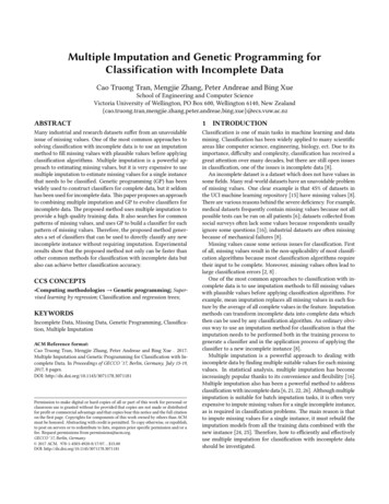
MULTIPLE IMPUTATION OF MISSING DATAMultiple Imputation is a robust and flexible option for handling missing data. For longitudinal data as wellas other data, MI is implemented following a framework for estimation and inference based upon a threestep process: 1) formulation of the imputation model and imputation of missing data using PROC MI witha selected method, 2) analysis of complete data sets using standard SAS procedures (that assume thedata are identically and independently distributed or from a simple random sample) or SURVEYprocedures for analysis of data from a complex sample design, and 3) analysis of the output from the twoprevious steps using PROC MIANALYZE (Berglund and Heeringa, 2014).A key assumption made in the MI and MIANALYZE procedures is that the missing data are missing atrandom (MAR) or in other words, the probability that an observation is missing depends on observed Ybut not missing Y, (Rubin, 1987).Two important advantages of multiple imputation are: 1) MI incorporates the variability introduced by theimputation during variance estimation and 2) MI offers use of appropriate statistical models for generatingplausible distributions of values to replace item-missing data. For more on multiple imputation and othertypes of imputation methods, see Schafer (1999), Rubin (1987) or more recently, Van Buuren (2012).MULTIPLE IMPUTATION METHODS FOR LONGITUDINAL DATAMI methods for longitudinal data can differ from those used to impute say, cross-sectional data. Typically,multiple records/values per respondent are included in longitudinal data sets (i.e. for each construct andtime point) and correlation among repeated records should be captured by the MI process.Longitudinal data is often collected in a long file format similar to Figure 1 where each respondent hasone or more records representing a key construct over time. In this simple example, income for 2 years iscollected in a multiple record per ID data format.Figure 1. Example of Long FileThe long format is convenient for data collection and analysis but may not be appropriate for multipleimputation, thus data restructuring from long to wide or the reverse is often needed for multiple imputationand subsequent MI analyses. For more on MI of longitudinal data and model assumptions, seeRaghunathan (2016) pages 121-126.“Just Another Variable” MethodA popular MI method used with longitudinal data is called “Just Another Variable” or JAV, (Raghunathan,2016). This method involves imputing missing data in a wide format data set with variables “strung out”one the data record. (See Figure 2). Though this method does not capture within-individual changesover time, it offers a convenient and flexible method for dealing with a varying number of records perindividual and differing time points for follow-up data collection. In addition, it is easily performed in SAS2
using PROC MI and PROC MIANALYZE. The JAV method is demonstrated in the analysis application inSection 2 of this paper.As the name suggests, this method treats each variable as “just another” to be imputed. For example,the long data format in Figure 1 can be easily restructured into a wide format where multiple records areturned into one record per unique ID with each construct and time (income and year respectively)represented by uniquely named variables (Income 2013 and Income 2015).Figure 2. Example of Long File Converted to Wide FormatThis data structure permits multiple imputation of item-missing data for each respondent’s uniquelynamed variables in the rectangular data array. Once imputation is finished, the wide data set is generally“reversed” back to the long format for subsequent analysis of imputed longitudinal data.Two-Fold Fully Conditional Specification MethodAn alternative imputation method for longitudinal data is the two-fold fully conditional specification(FCS) approach proposed by Welch, Bartlett, Peterson, (2014). This method performs a two step or “twofold” multiple imputation process outlined in Figure 3 (graphic adapted from Nevalainen, et al. (2009)).Figure 3. Diagram of Two-Fold Fully Conditional Specification ImputationFigure 3 highlights how the two-fold FCS method first imputes missing data within each wave (up/downarrows around each box in figure below) and secondly, imputes across waves using a user-specified t /(k) iterative process (horizontal arrows across top and bottom of figure). This method incorporates theimpact of each individual’s responses at time t, and those around t, by using t-k and t k, where k istypically 1 or 2 (specified by analyst).This method is not currently available in PROC MI but is discussed in detail in Nevalainen et al (2009).For more on the JAV and two-fold FCS methods, see De Silva, Moreno-Betancur, Madhu De Livera, Lee,and Simpson, (2017).3
PLANNING FOR MULTIPLE IMPUTATIONCareful planning of a multiple imputation session is critical to produce both high quality imputations andsubsequent analyses of imputed data sets. Often, the analyst is tempted to rush into multiple imputationwithout a complete understanding of the missing data problem and associated issues. The checklistpresented in Table 1 is a suggested guide for planning the multiple imputation project.Checklist of Issues and Considerations for the Multiple Imputation ProcessType of missing data - Item v. Unit, item missing data is topic of this presentation, unit generallyhandled by weighting adjustmentsAssumptions – Missing at Random (MAR default assumption of PROC MI/PROCMIANALYZE), Missing Completely at Random, Missing Not at RandomTypes of variables imputed - Continuous, nominal, binary, ordinal, count/mixedMissing data patterns - Arbitrary, monotone, file-matchingAmount of missing information - Extent of missing information is important factor whenselecting M (number of imputations)Imputation model - Imputation model(s) depends on type of variable(s) that require imputation(continuous, categorical, count, etc.), should include all analysis variables plus additional“auxilliary” variables to enrich imputation models (include complex sample design variables andweights too, if applicable), each variable to be imputed may have a different imputation modelNumber of imputations - Depends on how much data is missing, expected relative efficiency,how many records and variables included in imputation models, and other factors, may be aniterative process to evaluate M at certain numbers (say 10, 20, 25, 50.), if in doubt, use ahigher rather than lower MBig Data Imputation - Hardware/software limits, how many variables/records realistic toimpute/analyze, end-user capacities and analytic usage, burden on imputer and analystTable 1. Checklist of Issues and Considerations for the Multiple Imputation ProcessSECTION 2 - ANALYSIS APPLICATIONMULTIPLE IMPUTATION AND ANALYSIS OF LONGITUDINAL SURVEY DATA FROM THEPANEL STUDY OF INCOME DYNAMICS (PSID)Data ManagementThe analysis application uses data from the Panel Study of Income Dynamics (PSID),https://psidonline.isr.umich.edu/. The PSID is a long-running (1968-present) longitudinal study of U.S.families. The source data for this example was downloaded from the PSID data center.The analysis application employs descriptive statistics and linear growth curve models to analyze thefamily head’s wages/salary over time (1997-2013, odd years) by completed college status (completedgrade 16 US education system) while using multiply imputed data in all analyses.The downloaded PSID data set was filtered to include individuals that meet all three conditions, n 2.267: Individuals must be the family head in each odd year from 1997-2013 (9 waves of data), From either the Survey Research Center (SRC) or U.S. Census (Census) samples from 1968, Head must be present in family in each year of series.4
Prior to multiple imputation of item-missing data and subsequent analysis of completed data sets, somedata management was needed. The data from the PSID data center was structured as a wide file,therefore no transposition was required for imputation of missing data. However, previously imputedvalues (done by PSID staff using a modified “hotdeck” imputation method) were returned to their originalmissing data values with the goal of using the preferred multiple imputation method rather than thehotdeck method.A few additional variables were created for use in the multiple imputation process. For example, thenatural log of head’s wages/salary was created to address non-normal distributions, a combined Stratumand Sampling Error Computing Unit (SECU) or PSU variable was constructed to incorporate the impact ofthe PSID complex sample design stratification/clustering features in the imputation models, and a seriesof imputation “flag” variables were created to identify imputed values and assist in imputation diagnostics.For more on inclusion of complex sample design variables in multiple imputation, see Berglund andHeeringa (2014) or Reiter, Raghunathan, and Kinney (2006). Note that the SAS code for preliminary datamanagement is not shown here but available from the author upon request.The filtered, analysis data set includes the variables listed in Table 2, n 2,267. Note that age, education(highest grade completed), and log head’s wages/salary include a uniquely named variable for each ofnine waves of data used in the analysis application. The other variables are time-invariant and do notrequire strings of uniquely named variables. Also, variables highlighted in red have some missing data.Contents of Final MI Data Set (Wide Format)Er32000 - Gender (1 M, 2 F), fully observedAge1-Age9 - Age in 1997, 1999, 2001, 2003, 2005, 2007, 2009, 2011, 2013, fully observedStrat psu – Combined stratum and SECU (PSU) variable, fully observed, used toincorportate complex sample design features in imputation modelEr34268 – Probability weight from 2013, fully observedEd1-Ed9 – Highest grade completed (odd years 1997- 2013), missing data on eachvariableLoghdwg1-Loghdwg9 – Log of head’s wages/salary (odd years 1997-2013), missingdata on each variableID – ID68 and Person number combined to create unique individual indentifier, fully observedSamplecat – Sample indicator of SRC or Census (1968 original sample), fully observed dataTable 2. Contents of Final Analysis Data SetMULTIPLE IMPUTATION AND ANALYSIS PROCESSPrior to a detailed presentation of analysis examples, a brief outline of the MI process is provided.Step 1 Multiple Imputation of Missing DataStep 1 includes evaluation of the missing data problem, multiple imputation of missing data using PROCMI with the Fully Conditional Specification (FCS) method and other options/statements, and evaluation ofimputations using diagnostic tools such as plots and comparisons of observed versus imputed values.Once the imputations are considered final, the imputed data set is converted from a wide to long formatsuitable for longitudinal MI data analysis.Step 2 Analysis of Completed Data SetsStep 2 consists of analysis of the long, imputed data set using either standard (based SRS samples) orSURVEY procedures designed for analysis of complex sample data. The examples presented in this5
paper use standard procedures despite the complex sample design of the PSID. This is done to keepanalysis examples relatively simple, however a repeat of Example 2 using SAS-callable IVEware withSASMOD is presented in Appendix B.IVEware is a tool that can perform multiple imputation and analysis of imputed data while also handlingcomplex sample design variance estimation. The software and documentation is freely available fromiveware.org. The SASMOD command uses the correct combining rules for multiply imputed data andalso implements Jackknife Repeated Replication (Rust, 1985) for design-based variance estimation.Selected SAS procedures such as PROC MIXED, PROC GENMOD and others can be used withSASMOD framework. This additional complexity is needed only for analysis of data derived from complexsamples and also for SAS procedures such as PROC MIXED that do not have an equivalent SASSURVEY procedure.Step 3. Combine ResultsPROC MIANALYZE combines the results of MI Steps 1 and 2 and generates valid statistical inferencesby accounting for the variability introduced by the MI process.THREE- STEP MULTIPLE IMPUTATION PROCESSStep 1- Multiple Imputation of Missing DataEvaluation of Missing Data ProblemPrior to imputation, evaluation of the extent of the missing data problem, types of variables to be imputedor used in imputation models, and the pattern of missing data is recommended.Two approaches are demonstrated in the analysis examples: use of 1) PROC MEANS to examine eachvariable’s observed n (n), number missing (nmiss), and mean, minimum, and maximum values and 2)PROC MI with NIMPUTE 0 to obtain a missing data patterns grid without imputation. Both approachesassist with evalulation of the missing data problem prior to multiple imputation:proc means data w.psid1 n nmiss mean min max;var er32000 age1-age9 strat psu er34268 ed1-ed9 loghdwg1-loghdwg9;run;proc mi data w.psid1 nimpute 0;var er32000 age1-age9 strat psu er34268 ed1-ed9 loghdwg1-loghdwg9;run;PROC MEANS output is presented in Figure 4 and indicates missing data on each of the 9 educationvariables (ED1-ED9) and 9 log head’s wages/salary variables (LOGHDWG1-LOGHDWG9). All othervariables are fully observed.6
Figure 4. Results from PROC MEANSThe education variables (ED1-ED9) represent highest grade completed and are treated as continous.The continuous log head’s wages/salary variables (LOGHDWG1-LOGHDWG9) represent theprevious year’s wages/salary and range from 0 (did not receive wage/salary in dollars for a givenyear) to 15.06, on the log scale.We acknowlege that log-transformed variables can produce bias and heavy tails in the distribution ofthe back-transformed, imputed version but we proceed with the transformation as recent researchhas demonstrated that for regression estimates, this bias is often mild, von Hippel (2013). Anotherimportant caution is that age and time are linked and if age is used as a predictor in growth models, itshould be treated as time-invariant, e.g., age at a fixed point such as age in 1997.Figure 5 presents part of the Missing Data Patterns Grid produced by PROC MI. The grid providesfrequency counts/percentages for observed data (“X”) and missing data (“.”), for each variable to beused in multiple imputation models.Figure 5. Results from PROC MI7
There are 128 unique groups of missing/observed data combinations with just the first four presentedhere. Group 1 is defined as fully observed on all variables, i.e. 80.06% of sample or 1815 individuals areassigned to the complete data group while the entire grid identifies an additional 127 missing datapatterns each with 1.5% missing data, with an arbitrary missing data pattern.Based on Figures 4 and 5, the missing data problem is understood. For example, there are 18continuous variables that require imputation (constituting 20% of full data set), the fully observedvariables are a mix of continuous and categorical variables, and the missing data pattern is arbitrary. Thisinformation helps determine proper settings in the PROC MI code for multiple imputation.Multiple Imputation using PROC MINext, multiple imputation of missing data is performed by PROC MI with a number of statements andoptions. In the code below, the SEED 2017 option ensures the ability to replicate results at a later time,NIMPUTE 10 requests SAS create M 10, OUT IMPUTE PSID MI saves a vertically stacked, imputeddata set for subsequent use, ROUND () formats imputed values for each corresponding variable in theVAR statement, the BY SAMPLECAT statement imputes missing values separately within the PSID SRCand Census samples, a CLASS statement declares ER32000 and STRAT PSU as classificationvariables, FCS REGPMM selects the FCS Predicted Mean Matching method to impute missing data withNBITER 20 burn-in iterations and K 8 nearest neighbors, the (PLOTS TRACE) option requestsdiagnostic trace plots for LOGHDWG1-LOGHDWG9, and the VAR statement lists variables to be includedin the imputation models, ordered from no missing data to most missing, moving from left to right:proc mi data w.psid1seed 2017nimpute 10out impute psid miround . . . . . . . . . . . . 1 1 1 1 1 1 1 1 1 .01 .01 .01 .01 .01 .01.01 .01 .01 ;by samplecat ;class er32000 strat psu ;fcs nbiter 20 regpmm(ed1-ed9 / k 8 ) ;fcs nbiter 20 plots trace regpmm(loghdwg1-loghdwg9 / k 8 );var er32000 age1-age9 strat psu er34268 ed1-ed9 loghdwg1-loghdwg9 ;run;Multiple Imputation DiagnosticsFigures 6 and 7 present Trace plots of the 2004 head’s wages/salary imputation. Because theimputations were done separately for the SRC and Census samples, we evaluate each plot separately.Trace plots are typically used to detect non-random patterns that may arise during the imputationprocess. Random variation around imputed values, once burn-in iterations are complete, generallyindicates a lack of problems with the imputations.8
Figure 6. Trace Plot of Head’s Wages/Salary 2004, SRC SampleFigure 7. Trace Plot of Head’s Wages/Salary 2004, Census SampleBased on the random patterns of Figures 6 and 7, there is little concern about the quality of theseimputations. Detailed evaluation of all 18 plots produced by PROC MI (not shown here) also indicates noissues with the imputations.Alternatively, evaluation of imputations can be carried out by checking mean head’s wages/salary bySAMPLECAT, IMPUTATION (the automatic variable indicating imputation number), and the userdefined imputation flag, IMPHDWG1 (created in a previous DATA STEP):proc means data impute psid mi ;class samplecat imputation imphdwg1 ;var loghdwg1 ;run ;Figure 8 presents mean 1996 head’s wages/salary for 5 of 10 imputations by Census and SRC samples,imputation number, and imputation status. This diagnostic check also reveals no apparent issuesbetween observed (imphdwg1 0) versus imputed (imphdwg1 1) values.9
Figure 8. Mean Head’s Wages/Salary 1996 by Sample, Imputation, and Imputed StatusConvert Completed Data Sets from Wide to Long FormatPrior to analysis of completed data sets in MI Steps 2 and 3, the data is restructured into a long filecontaining 10 imputations*2,267 individuals*9 time points 204,030 records. The following DATA STEPcode demonstrates use of arrays with an iterative DO loop and OUTPUT statement to produce a multiplerecord per individual data set (9 waves per person) with back-transformed log head’s wages/salary andconversion to 2013 dollars:* Create a long data set with multiple records per person within eachimputed data set (identified by the imputation variable);data w.long imputed ;set impute psid mi ;if samplecat 'SRC' then src 1 ; else src 0 ;if er32000 2 then female 1 ; else female 0 ;id er30001*10000 er30002 ;* use arrays to output multiple records per individual ;array w [*] loghdwg1-loghdwg9 ;array ed [*] ed1-ed9 ;array cg [*] cg1-cg9 ;array y [9] temporary (1997 1999 2001 2003 2005 2007 2009 2011 2013) ;array wi [9] temporary (1.45 1.40 1.32 1.27 1.19 1.12 1.09 1.04 1.00) ;array t [9] temporary (1 2 3 4 5 6 7 8 9) ;array weight [*] er33430 er33546 er33637 er33740 er33848 er33950 er34045er34154 er34268 ;array ag [*] age1-age9 ;do i 1 to 9 ;hdwg exp (w[i]) ;headwage hdwg * wi[i] ;10
wgt weight[i];sex er32000;stratum er31996;cluster er31997;age ag[i];year y[i];time t[i] ;completeded ed[i] ;if ed[i] 16 then cg [i] 1 ; else cg [i] 0 ;collegegrad cg[i] ;mult imputation ;output ;end ;keep id hdwg headwage wgt sex stratum cluster age year time completededcollegegrad mult imputation er30001 er30002 er32000 samplecat er34268;run ;With the imputed, long data set now ready for MI analysis, detailed SAS code and results are presentedfor typical longitudinal analysis techniques.REVIEW OF ANALYSIS EXAMPLESThe primary analytic goal is to examine trends in head’s wages/salary over time by college graduationstatus. Both descriptive and regression techniques are used to address this goal.The descriptive analysis focuses on mean head’s wages/salary by year and college graduation status,produced by PROC MEANS and PROC GPLOT.Growth models are executed using PROC MIXED with a RANDOM statement to account for within andbetween-subject variation where predicted head’s wages/salary (based on mixed model results) arecalculated in the DATA STEP and then used in plots produced by PROC SGPLOT.As previously explained, Examples 1 and 2 ignore the PSID complex sample design features butincorporate all appropriate MI analysis and combining techniques. However, to provide guidance forthose working with complex sample data and multiply imputed data, Example 2 is repeated usingIVEware and the SASMOD command with PROC MIXED to compare how variances change when thecomplex sample design features of the PSID are incorporated. Results are presented in Appendix B.Analysis Example 1 - Mean Head’s Wages/Salary by Year and College Graduation StatusStep 2. Analysis of Completed Data SetsExample 1 inputs the long, imputed data set generated in MI Step 1 and demonstrates descriptiveanalysis of head’s wages/salary by imputation, college graduation status, and year. PROC MEANS isused to prepare summary statistics that are saved to an output data set for use in PROC MIANALYZE.The following code first sorts the LONG IMPUTED data set by IMPUTATION , COLLEGEGRAD, andTIME. Next, PROC MEANS with BY and WEIGHT statements is used to obtain weighted means ofhead’s wages/salary within each of 10 imputed data sets, by college status and time. The OUTPUTstatement saves the statistics of interest to a file called AVGWAGE and finally, PROC SORT sorts thedata for use in PROC MIANALYZE:proc sort data w.long imputed ;by imputation collegegrad time ;run ;11
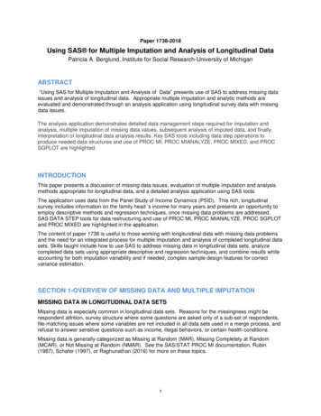
* Run PROC MEANS in long data set with 10*2267 (10 imputations) * 9 recordsper individual 204,030 ;proc means data w.long imputed mean stderr ;by imputation collegegrad time ;var headwage ;weight er34268 ;output out avgwage mean mean headwage stderr se headwage ;run ;proc print data avgwage ;run ;proc sort data avgwage ;by collegegrad time imputation ;run ;Step 3 – Combine ResultsPROC MIANALYZE combines results from Step 2 and generates variances that account for the additionalvariability introduced by the multiple imputation. These combined estimates are then used to plot meanwages/salary over time by college graduation status.The following code invokes PROC MIANALYZE and includes a BY statement to produce a combinedestimates by college status and time, MEAN HEADWAGE is declared as the MODELEFFECTS variable,SE HEADWAGE as the STDERR variable, and ODS OUTPUT saves an output data set with combined“parameter estimates” or means in this case, for use in PROC SGPLOT.PROC FORMAT creates descriptive labels for the plot, while PROC SGPLOT inputs the data set fromPROC MIANALYZE and uses SERIES, XAXIS, YAXIS, and FORMAT statements to customize the plotpresented in Figure 9:proc mianalyze data avgwage ;by collegegrad time ;modeleffects mean headwage ;stderr se headwage ;ods output parameterestimates outcombine 1 ;run ;proc format ;value tf 1 '1997' 2 '1999' 3 '2001' 4 '2003' 5 '2005' 6 '2007' 7 '2009'8 '2011' 9 '2013' ;value cf 0 'No' 1 'Yes' ;run ;proc sgplot data outcombine 1 ;title "Mean Head's Wages/Salary by College Graduate Status" ;series x time y estimate / group collegegrad markers ;xaxis label 'Year' ;yaxis label 'Mean Head Wage/Salary 1997 to 2013 (in 2013 Dollars)' ;format time tf. collegegrad cf. ;run ;12
Figure 9. Mean Head’s Wages/Salary by College Graduate Status, 1997-2013Figure 9 plots head’s wages/salary trends over time for college graduates and non-graduates andsuggests a possible interaction between year and college graduate status. For college graduates, thereis a mix of positive and sharp negative slopes while for non-graduates, the slopes are flatter/smaller andprimarily negative. The plot highlights trends as heads aged and experienced a changing economicclimate and other changes in their economic circumstances between 1997-2013. Furthermore, a wagedifferential of about 33,000 between college graduates and those that did not graduate from collegepersists over the years of interest.Analysis Example 2 – Growth ModelStep 2. Analysis of Completed Data SetsExample 2 demonstrates use of a growth model to investigate the impact of time and college graduationstatus on head’s wages/salary. This model accounts for between-subject (intercept) and within-subject(time) variation by requesting random intercepts and slopes while using time as a continuous rather thancategorical predictor, as in Example 1. As in the previous example, the long, imputed data set from Step1 is used as input for this example.Model Fitting Prior to InferencePrior to the inference step or Step 4 of the model building process, model fitting was performed byfollowing Steps 1-3 as recommended by the SAS Institute “Mixed Model Analyses of Repeated MeasuresData” course notes. (Results not shown but available upon request). Step 1- Model mean structure, specify fixed effects Step 2- Set covariance structure for within-subject and/or between-subject effects Step 3- Use Generalized Least Squares (GLS) to fit mean model with selectedcovariance structure Step 4- Make statistical inference based on Step 3, aim for parsimonious model13
To summarize, model fitting was done separately within each of the M 10 imputed data sets with 3covariance structures: 1) UN, 2) AR(1), and 3) Toeplitz. PROC MIANALYZE was used to combine resultsfor 10 imputed data sets/models and incorporate MI variability in variance estimates.After evaluation of the three covariance structures using AIC and BIC statistics, unstructured (UN)covariance was selected as the preferred structure for inference.Step 4 - InferenceThe following code uses PROC MIXED with a number of options and statements. Use of BYIMPUTATION executes a growth model within each of 10 imputed data sets, the CLASS statementtreats college graduation status and the respondent ID variable as classification variables, the MODELstatement uses HEADWAGE as a continous outcome with continuous TIME and the interaction ofTIME*COLLGEGRAD with a SOLUTION option to request fixed effects solutions and DDFM BW torequest the between-within method for computing denominator degrees of freedom, and a RANDOMINTERCEPT TIME / TYPE UN SUBJECT ID statement to request random intercepts and slopes with anunstructured covariance matrix. The PSID 2013 longitudinal weight is used in the WEIGHT statementwhile ODS OUTPUT requests an output data set of parameter estimates for use in PROC MIANALYZE.The final section of code uses PROC PRINT to show the contents of the output data setOUTCOMBINE RANDOM:*Step 4 Inference: Use RANDOM INTERCEPT/SLOPE with unstructured covariance;proc mixed data w.long imputed noclprint;by imputation ;class collegegrad id;model headwage time collegegrad time*collegegrad / solution ddfm bw;random intercept time / type un subject id;weight er34268;ods output solutionf outco
Multiple Imputation is a robust and flexible option for handling missing data. For longitudinal data as well as other data, MI is implemented following a framework for estimation and inference based upon a three step process: 1) formulation of the imputation model and imputation of missing data using PROC MI with