WIXLIB

MI is a simulation-based procedure. Its purpose is not to re-create the individual missing values asclose as possible to the true ones, but to handle missing data to achieve valid statistical inference(Schafer, 1997).It involves 3 steps:a) Running an imputation model defined by the chosen variables to create imputed data sets. Inother words, the missing values are filled in m times to generate m complete data sets. m 20 isconsidered good enough. Correct model choices require considering: Firstly, we should identify which are the variables with missing values. Secondly, we should compute the proportion of missing values for each variable. Thirdly, we should assess whether different missing value patterns exist in the data (SAShelps us doing this), and try to understand the nature of the missing values. Some keyquestions are:-Are there a lot of missing values for certain variables? (E.g. Sensitive question, dataentry errors?)-Are there groups of subjects with very little information available? (E.g. Do they havesomething in common?)-Which is the pattern of missingness? Monotone or arbitrary?b) The m complete data sets are analyzed by using standard proceduresc) The parameter estimates from each imputed data set are combined to get a final set of parameterestimates.Advantages: It has the same optimal properties as ML, and it removes some of its limitations. Multipleimputation can be used with any kind of data and model with conventional software. When the data isMAR, multiple imputation can lead to consistent, asymptotically efficient, and asymptotically normalestimates.Limitations: It is a bit challenging to successfully use it. It produces different estimates (hopefully, onlyslightly different) every time you use it, which can lead to situations where different researchers getdifferent numbers from the same data using the same method (Nakai & Weiming, 2011), (Allison,2001).4.2.2.Maximum LikelihoodWe can use this method to get the variance-covariance matrix for the variables in the model based onall the available data points, and then use the obtained variance- covariance matrix to estimate ourregression model (Schafer, 1997).Page 8

Compared to MI, MI requires many more decisions than ML (whether to use Markov Chain Monte Carlo(MCMC) method or the Fully Conditional Specification (FCS), how many data sets to produce, how manyiterations between data sets, what prior distribution to use-the default is Jeffreys-, etc.). On the other hand,ML is simpler as you only need to specify your model of interest and indicate that you want to use ML ( SASInstitute, 2005).There are two main ML methods:a) Direct Maximum Likelihood: It implies the direct maximization of the multivariate normallikelihood function for the assumed linear model. Advantage: It gives efficient estimates withcorrect standard errors. Limitations: It requires specialized software (it may be challengingand time consuming).b) The Expectation-maximization (EM) algorithm: It provides estimates of the means andcovariance matrix, which can be used to get consistent estimates of the parameters of interest.It is based on an expectation step and a maximization step, which are repeated several timesuntil maximum likelihood estimates are obtained. It requires a large sample size and that thedata are missing at random (MAR). Advantage: We can use SAS, since this is the defaultalgorithm it employs for dealing with missing data with Maximum Likelihood. Limitations: Onlycan be used for linear and log-linear models (there is neither theory nor software developedbeyond them). (Allison, 2001) (Graham, 2009) (Enders & Bandalos, 2001) and (Allison, 2003).4.3.Other advanced methods4.3.1.Bayesian simulation methodsThere are two main methods:a) Schafer algorithms: It uses Bayesian iterative simulation methods to impute data sets assumingMAR. Precisely, it splits the multivariate missing problem into a series of univariate problems based onthe assumed distribution of the multivariate missing variables (e.g. multivariate normal for continuousvariables, multinomial loglinear for categorical variables). In other words, it uses an iterative algorithmthat draws samples from a sequence of univariate regressions.b) Van Buuren algorithm: It is a semi-parametric approach. The parametric part implies that eachvariable has a separate imputation model with a set of predictors that explain the missingness. Thenon-parametric part implies the specification of an appropriate form (e.g. linear), which depends on thePage 9

kind of variables (Briggs et al., 2003) (Kong et al., 1994).4.3.2.Hot deck imputation methodsIt is used by the US Census Bureau. This method completes a missing observation by selecting atrandom, with replacement, a value from those individuals who have matching observed values forother variables. In other words, a missing value is imputed based on an observed value that is closerin terms of distance.SAS macro developed by Lawrence Altmayer, of the U.S. Census Bureau. Can befound in Ahmed Kazi et al; 2009. (Briggs et al., 2003).5. Dealing with missing data using SASFor illustrative purposes, I will use a data set constructed to analyze the socioeconomic determinantsof health in the OCDE (32 countries) from 1980-2010 (in 5 year intervals). The dependent variable ofinterest is the Health Index, which is part of the United Nations Human Development Index. Theexplanatory variables are the growth rate of the GDP per capita, the unemployment rate, the inequalityin the distribution of wealth (measured by the Gini coefficient), and 3 dummy variables capturing thelevel of social and health expenditure and the existence of a National Health System. There are 88missing values in the dataset, whichreduces the sample size from 224 to 136observations.The variables with missing values are GINIcoefficient, GDP and Unemployment (U).Page 10

5.1.Multiple Imputation (MI)There are several imputation methods in PROC MI. The method of choice depends on thepattern of missingness in the data and the type of the imputed variable, as the table belowsummarizes:Pattern of missingnessType of imputed variableAvailable MethodsContinuous )Monotone regression2)Monotone predicted mean matching ores:Monotone propensity score.Ordinal Monotone logistic regressionNominal Monotone discriminant functionContinuous Markov Chain Monte Carlo (MCMC) full-data imputation MCMC monotone-data imputation Fully conditional specification (FCS), which assumes theexistence of a joint distribution for all variables. FCS regressionArbitrary FCS predicted mean matchingOrdinal FCS logistic regressionNominal FCS discriminant functionSource: Table modified from “The MI Procedure Imputation Methods, SAS 9.3, The SAS dl/en/statug/63962/HTML/default/viewer.htm#statug mi sect019.htmIn our case, the pattern of missingness is arbitrary and all variables with missing values are continuous. Wechoose MCMC full-data imputation, which uses a single chain to create 5 imputations. The posterior mode,the highest observed-data posterior density, with a noninformative prior, is computed from theexpectation-maximization (EM) algorithm and is used as the starting value for the chain.proc mi data Final seed 501213 out outmi;mcmc;var GDP GINI U;run;Page 11

Description of the output:200 burn-in iterations were usedbefore the first imputation and 100iterations between imputation,which are used to eliminate theseries of dependence between thetwo imputationsIt lists different missing data patterns with the corresponding frequency and percentage theyrepresent. ‘X’ implies that the variable is observed, while ‘.’ that it is missing. Group means arealso displayed.It presents the between-imputation variance, within-imputation variance, and total variance forcombining complete-data inferences for each variable, along with the degrees of freedom for thetotal variance.Page 12

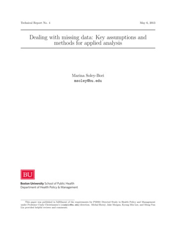
It summarizes basic descriptive statistics for the imputed values by variable.The imputed data sets are stored in the outmi data set, with the index variable Imputation indicating theimputation numbers. The data set can now be analyzed using standard statistical procedures with Imputation asa BY variable (Yuan, 2011) and (http://www.ats.ucla.edu/stat/sas/seminars/missing data/part1.htm).5.2.Maximum Likelihood (ML)We consider two options to deal with missing values on the independent variables:a) The EM algorithm in PROC MIPROC MI uses the default algorithm (EM) to do maximum likelihood of the means and thecovariance matrix and, then, it considers these estimates as starting values for multiple imputationalgorithms. We can use the estimates obtained on the first step.proc mi data Final nimpute 0;This option suppresses multiple imputationvar HI GDP U GINI SE NHS HE;It requests EM (expectation-maximization) estimates andem outem Finalem;writes the means and covariance matrix into a SAS datarun;set called ‘Finalem’Next, we use the output data set from PROC MI (the EM covariance matrix) as input to PROC REGto estimate our model:proc reg data Finalem;model HI GDP U GINI SE NHS HE;run;Page 13

The parameter estimates are the true maximum likelihood estimates of the regression coefficients, so wehave accomplished our goal.However, p-values are useless (we get a warning from SAS saying so). Solution: estimate the standard errorsand p-values by bootstrapping1.b) The “full-information” maximum likelihood method in PROC CALISAdvantage: Single procedure available in SAS 9.2.It is maximum likelihood estimation adjusting for the cases with missing data, which is called ‘FullInformation Maximum Likelihood’ (FIML) or ‘Direct Maximum Likelihood’.PROC CALIS was originally designed to estimate Structural Equation Models and its defaultestimation method is maximum likelihood under the assumption of multivariate normality.proc calis data Final method fiml;Specifying METHOD FIML thepath HI - GDP U GINI SE NHS HE;missing values are also considered.run;Notice that in this method we are making the same assumptions as with PROC MI (missing atrandom and multivariate normality). Also, it can handle almost any linear model.Disadvantage: It cannot deal with logistic regression (dependent dichotomous variable) ornegative binomial regression (count data). In these cases, we have to use MI.(Yuan, sing data/part1.htm)1It involves: 1) From the original sample size N, draw many samples of size N with replacements, 2) Obtain the EMestimates of the means/covariance matrix for each sample, 3) Estime the regression model from each covariancematrix, 4) Compute the standard deviation of each regression coefficient across samples.Page 14

6. Dealing with missing data using STATA6.1.Multiple imputationBasic steps:1) Declare the data to be ‘mi’ data:use datasetmi set mlong*On the last statement, we choose the data in marginallong style (mlong)-a memory efficient style*2) Register all variables relevant for the analysis as imputed, passive or regularmi register imputed v1mi register regular v2 v3 v4*v1 is the only one with missing data*3) Imputate the missing valuesmi impute regress v1 v2 v3 v4, add(20) ption). We also specify the rseed() option forreproducibility.4) Check that the imputation was done correctly: Compute basic descriptive statistics of v1for some imputations (e.g. m 0 -the one with missing values-, m 1 and m 20)mi xeq 0 1 20: summarize v15) Run the analysis using the mi estimate prefix commandmi estimate, dots: logit v1 v2 v3 v46.2.Other imputation methods available in STATA Hot deck imputation: Sg116 Weighted logistic regression for data with missing values using the mean score method:Sg156Page 15

Imputed values by best sub-set regression: ‘ Impute’ procedureIt involves 3 steps: 1) Identify all of the possible regression models derived from all of thepossible combinations of the candidate predictors, 2) from the possible models identified inthe first step, determine the one-predictor models that do the "best" at meeting somewell-defined criteria, the two-predictor models that do the "best, the three-predictor modelsthat do the "best," and so on. 3) Further evaluate and refine the handful of models identified inthe last step. More stat501/node/89 (StataCorp, 2009)Final question: What if our data is missing but not at random? We must specify a model for theprobability of missing data, which can be pretty challenging as it requires a good understanding of the datagenerating process. The Sample Selection Bias Model, by James Heckman, is a widely used method thatyou can apply in SAS using PROC QLIM (Heckman et al., 1998). The motivating example for this approachis a regression that predicts women’s wages, where wages data are missing for women who are not in thelabor market force. Those women who know that their wages will be very low based on their education andprevious job experience may be less likely to enter the job market. Thus, the data are not missing at random(Allison, 2002).7. Other software SOLAS http://www.solasmissingdata.com/software , SPSS s-missing-values/ S-PLUS g.pdfPage 16

8. Sources and useful resources8.1.OverviewAllison, P., 2001. Missing data — Quantitative applications in the social sciences. Thousand Oaks, CA:Sage. Vol. 136. A very useful book to understand both the theoretical and practical implications of thedifferent methods to deal with missing data.Briggs, A., Clark, T., Wolstenholme, J., Clarke, P., 2003. Missing. presumed at random: cost-analysis ofincomplete data. Health Economics 12, 377–392. A great article to get an overview of the differentmethods (including advanced methods such as Bayesian simulation methods) and assumptions. It alsoincludes a useful example about missing data imputation in cost datasets.Graham, J.W., 2009. Missing data analysis: making it work in the real world. Annu Rev Psychol 60,549–576. It presents an excellent summary of the main missing data literature. Solutions are given formissing data challenges such as handling longitudinal, categorical, and clustered dataNakai M and Weiming Ke., 2011. Review of Methods for Handling Missing Data in Longitudinal DataAnalysis. Int. Journal of Math. Analysis. Vol. 5, no.1, 1-13. It reviews and discusses general approachesfor handling missing data in longitudinal studiesSAS Institute, 2005. Multiple Imputation for Missing Data: Concepts and New Approaches. A usefuloverview of the different methods to deal with missing data using SAS.Schafer, J. L. ,1997. Analysis of Incomplete Multivariate Data, New York: Chapman and Hall Excellentbook aimed at bridging the gap between theory and practice. It presents a unified, Bayesian approach to theanalysis of incomplete multivariate data.STATA 11, 2009, Multiple Imputation.StataCorp. Comprehensive manual for dealing with missing datausing STATA. It provides many useful examples and detailed explanations.Yuan Yang C., 2011. Multiple imputation for Missing Data: Concepts and New Development (SAS Version9.0). SAS Institute Inc., Rockville, MA). A useful overview of the different methods to deal with missingdata using SAS.Page 17

8.2.AdvancedAhmed K, et al., 2009.Applying Missing Data Imputation Methods to HOS Household Income Data.Prepared by the National Committee for Quality Assurance (NCQA) for the Centers for Medicare andMedicaid ServicesAllison P., 2000. Multiple imputation for missing data. A caution tale. Sociological Methods and Research,Vol. 28, No.3.Allison P., 2003. Handling Missing Data by Maximum Likelihood. SAS Global Forum 2012. Development(Version 9.0)Heckman, J., Ichimura, H., Smith, J., Todd, P., 1998. Characterizing Selection Bias Using ExperimentalData. Econometrica 66, 1017–1098.Enders, C.K., Bandalos, D.L., 2001. The Relative Performance of Full Information Maximum LikelihoodEstimation for Missing Data in Structural Equation Models. Structural Equation Modeling: A MultidisciplinaryJournal 8, 430–457.Kong A., Liu KJ and Hung Wong W., 1994. Sequential Imputations and Bayesian Missing Data Problems.Journal of the American Statistical Association 89, 425, 278-288Rubin, D.B., 1976. Inference and missing data. Biometrika 63, 581–592.STATA. Multiple –Imputation Reference Manual. 2009.Twisk, J., De Vente, W., 2002. Att

reviewed, including Listwise deletion, Imputation methods, Multiple Imputation, Maximum Likelihood and Bayesian methods. Advantages and limitations are specified so that the reader is able to identify the main trade-offs when using each method. The report also summarizes how to carry out Multiple Imputation and Maximum Likelihood using SAS and .